See also, Basic Notations and Principles.

Data Mining. StatSoft defines data mining as an analytic process designed to explore large amounts of (typically business or market related) data in search for consistent patterns and/or systematic relationships between variables, and then to validate the findings by applying the detected patterns to new subsets of data. Data mining uses many of the principles and techniques traditionally referred to as Exploratory Data Analysis (EDA). For more information, see Data Mining.
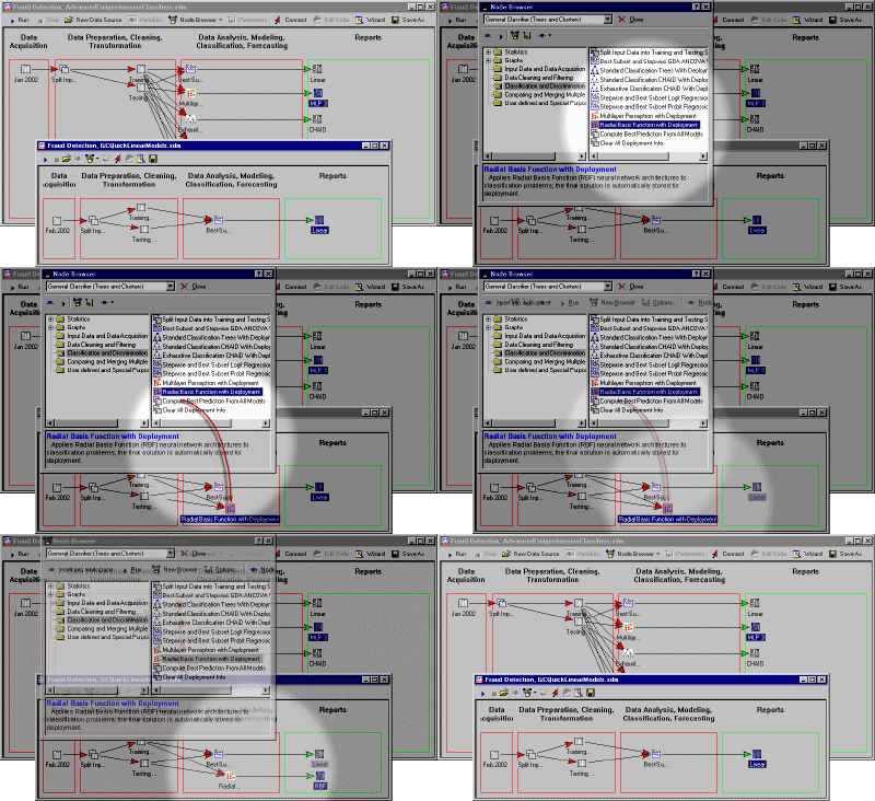
Data Preparation Phase. In Data Mining, the input data are often "noisy," containing many errors, and sometimes information in unstructured form (e.g., in Text Mining). For example, suppose you wanted to analyze a large database of information collected on-line via the web, based on voluntary responses of persons reviewing your web site (e.g., potential customers of a web-based retailer, who filled out suggestion forms). In those instances it is very important to first verify and "clean" the data in a data preparation phase, before applying any analytic procedures. For example, some individuals might enter clearly faulty information (e.g., age = 300), either by mistake or intentionally. If those types of data errors are not detected prior to the analysis phase of the data mining project, they can greatly bias the result, and potentially cause unjustified conclusions. Typically, during the data preparation phase, the data analyst applies "filters" to the data, to verify correct data ranges, and to delete impossible co-occurrences of values (e.g., Age=5; Retired=Yes).

Data Reduction. The term Data Reduction is used in two distinctively different meanings:

Data Reduction by decreasing the dimensionality (exploratory multivariate statistics). This interpretation of the term Data Reduction pertains to analytic methods (typically multivariate exploratory techniques such as Factor Analysis, Multidimensional Scaling, Cluster Analysis, Canonical Correlation, or Neural Networks) that involve reducing the dimensionality of a data set by extracting a number of underlying factors, dimensions, clusters, etc., that can account for the variability in the (multidimensional) data set. For example, in poorly designed questionnaires, all responses provided by the participants on a large number of variables (scales, questions, or dimensions) could be explained by a very limited number of "trivial" or artifactual factors. For example, two such underlying factors could be: (1) the respondent's attitude towards the study (positive or negative) and (2) the "social desirability" factor (a response bias representing a tendency to respond in a socially desirable manner).

Data Reduction by unbiased decreasing of the sample size (exploratory graphics). This type of Data Reduction is applied in exploratory graphical data analysis of extremely large data sets. The size of the data set can obscure an existing pattern (especially in large line graphs or scatterplots) due to the density of markers or lines. Then, it can be useful to plot only a representative subset of the data (so that the pattern is not hidden by the number of point markers) to reveal the otherwise obscured but still reliable pattern. For an animated illustration, see the Data Reduction section of the Selected Topics in Graphical Analytic Techniques chapter.

Data Rotation (in 3D space). Changing the viewpoint for 3D scatterplots (e.g., simple, spectral, or space plots) may prove to be an effective exploratory technique since it can reveal patterns that are easily obscured unless you look at the "cloud" of data points from an appropriate angle (see the animation below).

Rotating or spinning a 3D graph will allow you to find the most informative location of the "viewpoint" for the graph. For more information see the section on Data Rotation (in 3D space) in the Graphical Techniques chapter.

Data Warehousing. StatSoft defines data warehousing as a process of organizing the storage of large, multivariate data sets in a way that facilitates the retrieval of information for analytic purposes.

For more information, see Data Warehousing.

Degrees of Freedom. Used in slightly different senses throughout the study of statistics, Degrees of Freedom were first introduced by Fisher based on the idea of degrees of freedom in a dynamical system (e.g., the number of independent co-ordinate values which are necessary to determine it). The degrees of freedom of a set of observations are the number of values which could be assigned arbitrarily within the specification of the system. For example, in a sample of size n grouped into k intervals, there are k-1 degrees of freedom, because k-1 frequencies are specified while the other one is specified by the total size n. Thus in a p by q contingency table with fixed marginal totals, there are (p-1)(q-1) degrees of freedom. In some circumstances the term degrees of freedom is used to denote the number of independent comparisons which can be made between the members of a sample.

Deleted residual. The deleted residual is the residual value for the respective case, had it not been included in the regression analysis, that is, if one would exclude this case from all computations. If the deleted residual differs greatly from the respective standardized residual value, then this case is possibly an outlier because its exclusion changed the regression equation.

See also, standard residual value, Mahalanobis distance, and Cook’s distance.

Delta-Bar-Delta (in Neural Networks). Delta-bar-Delta (Jacobs, 1988; Patterson, 1996) is an alternative to back propagation, which is sometimes more efficient, although it can be more inclined to stick in local minima than back propagation. Unlike quick propagation, it tends to be quite stable.

Like quick propagation, Delta-bar-Delta is a batch algorithm: the average error gradient across all the training cases is calculated on each epoch, then the weights are updated once at the end of the epoch.

Delta-bar-Delta is inspired by the observation that the error surface may have a different gradient along each weight direction, and that consequently each weight should have its own learning rate (i.e. step size).

In Delta-bar-Delta, the individual learning rates for each weight are altered on each epoch to satisfy two important heuristics:

• If the derivative has the same sign for several iterations, the learning rate is increased (the error surface has a low curvature, and so is likely to continue sloping the same way for some distance);

• If the sign of the derivative alternates for several iterations, the learning rate is rapidly decreased (otherwise the algorithm may oscillate across points of high curvature).

To satisfy these heuristics, Delta-bar-Delta has an initial learning rate used for all weights on the first epoch, an increment factor  added to learning rates when the derivative does not change sign, and a decay rate multiplied by the learning rates when the derivative does change sign. Using linear growth and exponential decay of learning rates contributes to stability.

The algorithm described above could still be prone to poor behavior on noisy error surfaces, where the derivative changes sign rapidly even within an overall downward trend. Consequently, the increase or decrease of learning rate is actually based on a smoothed version of the derivative.

Technical Details. Weights are updated using the same formula as in back propagation, except that momentum is not used, and each weight has its own time-dependent learning rate.

All learning rates are initially set to the same starting value; subsequently, they are adapted on each epoch using the formulae below.

The bar-Delta value is calculated as:

d(t) is the derivative of the error surface,

q is the smoothing constant.

The learning rate of each weight is updated using:

k is the linear increment factor,

f the exponential decay factor.

For descriptions of denominator synthesis, see the Variance Components and Mixed-Model ANOVA/ANCOVA chapter and the General Linear Models chapter.

Deployment. The concept of deployment in predictive data mining refers to the application of a model for prediction or classification to new data. After a satisfactory model of set of models have been identified (trained) for a particular application, one usually wants to deploy those models so that predictions or predicted classifications can quickly be obtained for new data. For example, a credit card company may want to deploy a trained model or set of models (e.g., neural networks, meta-learner) to quickly identify transactions which have a high probability of being fraudulent.

Design Matrix. In general linear models and generalized linear models, the design matrix is the matrix X for the predictor variables which is used in solving the normal equations. X is a matrix, with 1 row for each case and 1 column for each coded predictor variable in the design, whose values identify the levels for each case on each coded predictor.

See also general linear model, generalized linear model.

Desirability Profiles. The relationship between predicted responses on one or more dependent variables and the desirability of responses is called the desirability function. Profiling the desirability of responses involves, first, specifying the desirability function for each dependent variable, by assigning predicted values a score ranging from 0 (very undesirable) to 1 (very desirable). The individual desirability scores for the predicted values for each dependent variable are then combined by computing their geometric mean. Desirability profiles consist of a series of graphs, one for each independent variable, of overall desirability scores at different levels of one independent variable, holding the levels of the other independent variables constant at specified values. Inspecting the desirability profiles can show which levels of the predictor variables produce the most desirable predicted responses on the dependent variables.

For a detailed description of response/desirability profiling see Profiling Predicted Responses and Response Desirability.

Detrended Probability Plots. This type of graph is used to evaluate the normality of the distribution of a variable, that is, whether and to what extent the distribution of the variable follows the normal distribution. The selected variable will be plotted in a scatterplot against the values "expected from the normal distribution." This plot is constructed in the same way as the standard normal probability plot, except that before the plot is generated, the linear trend is removed. This often "spreads out" the plot, thereby allowing the user to detect patterns of deviations more easily.

Deviance. To evaluate the goodness of fit of a generalized linear model, a common statistic that is computed is the so-called Deviance statistic. It is defined as:

Deviance = -2 * (Lm - Ls)

where Lm denotes the maximized log-likelihood value for the model of interest, and Ls is the log-likelihood for the saturated model, i.e., the most complex model given the current distribution and link function . For computational details, see Agresti (1996).

See also the description of Generalized Linear Models.

Deviance residuals. After fitting a generalized linear model to the data, to check the adequacy of the respective model, one usually computes various residual statistics. The deviance residual is computed as:

r_D = sign(y-µ)sqrt(d_i)

Where Sd_i = D, and D is the overall deviance measure of discrepancy of a generalized linear model (see McCullagh and Nelder, 1989, for details). Thus, the deviance statistic for an observation reflects it's contribution to the overall goodness of fit (deviance) of the model.

See also the description of the Generalized Linear Models chapter.

Deviation. In radial units, a figure multiplied by the radial exemplar's squared distance from the input pattern to generate the unit's activation level, before submission to the activation function. See neural networks.

Deviation Assignment Algorithms (in Neural Networks). These algorithms assign deviations to the radial units in certain network types. The deviation is multiplied by the distance between the unit's exemplar vector and the input vector, to determine the unit's output.  In essence, the deviation gives the size of the cluster represented by a radial unit.

Deviation assignment algorithms are used after radial centers have been set; see Radial Sampling and K Means.

Explicit Deviation Assignment. The deviation is set to an explicit figure provided by the user.

Notes. The deviation assigned by this technique is not the standard deviation of the Gaussians; it is the value stored in the unit threshold, which is multiplied by the distance of the weight vector from the input vector.  It is related to the standard deviation by:

Isotropic Deviation Assignment. This algorithm uses the isotropic deviation heuristic (Haykin, 1994) to assign the deviations to radial units. This heuristic attempts to determine a reasonable deviation (the same for all units), based upon the number of centers, and how spread out they are.

This isotropic deviation heuristic sets radial deviations to:

where d is the distance between the two most distant centers, and k is the number of centers.

K-Nearest Neighbor Deviation. The K-nearest neighbor deviation assignment algorithm (Bishop, 1995) assigns deviations to radial units by using the RMS (Root Mean Squared) distance from the K units closest to (but not coincident with) each unit as the standard deviation (assuming the unit models a Gaussian). Each unit hence has its own independently calculated deviation, based upon the density of points close to itself.

If less than K non-coincident neighbors are available, the algorithm uses the neighbors that are available.

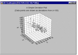
Deviation plots are similar to space plots. As compared to space plots, however in deviation plots the "deviations plane" is "invisible" and not marked by the location of the X-Y axes (those axes are always fixed in the standard bottom position). Deviation plots may help explore the nature of 3D data sets by displaying them in the form of deviations from arbitrary (horizontal) levels. Such "cutting" methods can help identify interactive relations between variables.

See also, Data Rotation (in 3D space) in the Graphical Techniques chapter.

DFFITS. Several measures have been given for testing for leverage and influence of a specific case in regression (including studentized residuals, studentized deleted residuals, DFFITS, and standardized DFFITS). Belsley et al. (1980) have suggested DFFITS, a measure which gives greater weight to outlying observations than Cook's distance. The formula for DFFITS is

DFFIT_i = _ie_i/(1-_i)

where
e_i    is the error for the ith case
h_i    is the leverage for the ith case

and _i = 1/N + h_i.

For more information see Hocking (1996) and Ryan (1997).

DIEHARD Suite of Tests and Random Number Generation. Many areas of statistical analysis, research, and simulation rely on the quality of random number generators. Most programs for statistical data analysis contain a function for generating uniform random numbers. A recent review of statistical packages (McCullough, 1998, 1999) that appeared in The American Statistician tested the random number generators of several programs using the so-called DIEHARD suite of tests (Marsaglia, 1998). DIEHARD applies various methods of assembling and combining uniform random numbers, and then performs statistical tests that are expected to be nonsignificant; this suite of tests has become a standard method of evaluating the quality of uniform random number generator routines.

Differencing (in Time Series). In this Time Series transformation, the series will be transformed as: X=X-X(lag). After differencing, the resulting series will be of length N-lag (where N is the length of the original series).

Dimensionality Reduction. Data Reduction by decreasing the dimensionality (exploratory multivariate statistics). This interpretation of the term Data Reduction pertains to analytic methods (typically multivariate exploratory techniques such as Factor Analysis, Multidimensional Scaling, Cluster Analysis, Canonical Correlation, or Neural Networks) that involve reducing the dimensionality of a data set by extracting a number of underlying factors, dimensions, clusters, etc., that can account for the variability in the (multidimensional) data set. For more information, see Data Reduction.

Discrepancy Function. A numerical value that expresses how badly a structural model reproduces the observed data. The larger the value of the discrepancy function, the worse (in some sense) the fit of model to data. In general, the parameter estimates for a given model are selected to make a discrepancy function as small as possible.

The discrepancy functions employed in structural modeling all satisfy the following basic requirements:

1. They are non-negative, i.e., always greater than or equal to zero.
2. They are zero only if fit is perfect, i.e., if the model and parameter estimates perfectly reproduce the observed data.
3. The discrepancy function is a continuous function of the elements of S, the sample covariance matrix, and (), the "reproduced" estimate of S obtained by using the parameter estimates and structural model.

Discriminant Function Analysis. Discriminant function analysis is used to determine which variables discriminate between two or more naturally occurring groups (it is used as either a hypothesis testing or exploratory method). For example, an educational researcher may want to investigate which variables discriminate between high school graduates who decide (1) to go to college, (2) to attend a trade or professional school, or (3) to seek no further training or education. For that purpose the researcher could collect data on numerous variables prior to students' graduation. After graduation, most students will naturally fall into one of the three categories. Discriminant Analysis could then be used to determine which variable(s) are the best predictors of students' subsequent educational choice (e.g., IQ, GPA, SAT).

For more information, see the Discriminant Function Analysis chapter; see also the Classification Trees chapter.

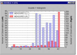
Double-Y Histograms. The Double-Y histogram can be considered to be a combination of two separately scaled multiple histograms. Two different series of variables can be selected. A frequency distribution for each of the selected variables will be plotted but the frequencies of the variables entered into the first list (called Left-Y variables) will be plotted against the left-Y axis, whereas the frequencies of the variables entered into the second list (called Right-Y variables) will be plotted against the right-Y axis. The names of all variables from the two lists will be included in the legend followed by a letter L or R, denoting the Left-Y and Right-Y axis, respectively.

This graph is useful to compare distributions of variables with different frequencies.

Drill-Down Analysis. The concept of drill-down analysis applies to the area of data mining, to denote the interactive exploration of data, in particular of large databases. The process of drill-down analyses begins by considering some simple break-downs of the data by a few variables of interest (e.g., Gender, geographic region, etc.). Various statistics, tables, histograms, and other graphical summaries can be computed for each group. Next one may want to "drill-down" to expose and further analyze the data "underneath" one of the categorizations, for example, one might want to further review the data for males from the mid-west. Again, various statistical and graphical summaries can be computed for those cases only, which might suggest further break-downs by other variables (e.g., income, age, etc.). At the lowest ("bottom") level are the raw data: For example, you may want to review the addresses of male customers from one region, for a certain income group, etc., and to offer to those customers some particular services of particular utility to that group.

Dunnett's test. This post hoc test (or multiple comparison test) can be used to determine the significant differences between a single control group mean and the remaining treatment group means in an analysis of variance setting. Dunnett's test is considered to be one of the least conservative post hoc tests (for a detailed discussion of different post hoc tests, see Winer, Michels, & Brown (1991). For more details, see the General Linear Models chapter. See also, Post Hoc Comparisons. For a discussion of statistical significance, see Elementary Concepts.

DV. DV stands for Dependent Variable. See also Dependent vs. Independent Variables.