Basic Ideas: The General Linear Model
The following topics summarize the historical, mathematical, and computational foundations for the general linear model. For a basic introduction to ANOVA (MANOVA, ANCOVA) techniques, refer to the the ANOVA/MANOVA chapter; for an introduction to multiple regression, see the Multiple Regression chapter; for an introduction to the design an analysis of experiments in applied (industrial) settings, see also the Experimental Design chapter.
The roots of the general linear model surely go back to the origins of mathematical thought, but it is the emergence of the theory of algebraic invariants in the 1800's that made the general linear model, as we know it today, possible. The theory of algebraic invariants developed from the groundbreaking work of 19th century mathematicians such as Gauss, Boole, Cayley, and Sylvester. The theory seeks to identify those quantities in systems of equations which remain unchanged under linear transformations of the variables in the system. Stated more imaginatively (but in a way in which the originators of the theory would not consider an overstatement), the theory of algebraic invariants searches for the eternal and unchanging amongst the chaos of the transitory and the illusory. That is no small goal for any theory, mathematical or otherwise.
The wonder of it all is the theory of algebraic invariants was successful far beyond the hopes of its originators. Eigenvalues, eigenvectors, determinants, matrix decomposition methods; all derive from the theory of algebraic invariants. The contributions of the theory of algebraic invariants to the development of statistical theory and methods are numerous, but a simple example familiar to even the most casual student of statistics is illustrative. The correlation between two variables is unchanged by linear transformations of either or both variables. We probably take this property of correlation coefficients for granted, but what would data analysis be like if we did not have statistics that are invariant to the scaling of the variables involved? Some thought on this question should convince you that without the theory of algebraic invariants, the development of useful statistical techniques would be nigh impossible.
The development of the linear regression model in the late 19th century, and the development of correlational methods shortly thereafter, are clearly direct outgrowths of the theory of algebraic invariants. Regression and correlational methods, in turn, serve as the basis for the general linear model. Indeed, the general linear model can be seen as an extension of linear multiple regression for a single dependent variable. Understanding the multiple regression model is fundamental to understanding the general linear model, so we will look at the purpose of multiple regression, the computational algorithms used to solve regression problems, and how the regression model is extended in the case of the general linear model. A basic intruction to multiple regression methods, and the analytic problems to which they are applied, is also provided in the Multiple Regression chapter.
| To index |
The Purpose of Multiple Regression
The general linear model can be seen as an extension of linear multiple regression for a single dependent variable, and understanding the multiple regression model is fundamental to understanding the general linear model. The general purpose of multiple regression (the term was first used by Pearson, 1908) is to quantify the relationship between several independent or predictor variables and a dependent or criterion variable. For a detailed introduction to multiple regression, also refer to the Multiple Regression chapter. For example, a real estate agent might record for each listing the size of the house (in square feet), the number of bedrooms, the average income in the respective neighborhood according to census data, and a subjective rating of appeal of the house. Once this information has been compiled for various houses it would be interesting to see whether and how these measures relate to the price for which a house is sold. For example, one might learn that the number of bedrooms is a better predictor of the price for which a house sells in a particular neighborhood than how "pretty" the house is (subjective rating). One may also detect "outliers," for example, houses that should really sell for more, given their location and characteristics.
Personnel professionals customarily use multiple regression procedures to determine equitable compensation. One can determine a number of factors or dimensions such as "amount of responsibility" (Resp) or "number of people to supervise" (No_Super) that one believes to contribute to the value of a job. The personnel analyst then usually conducts a salary survey among comparable companies in the market, recording the salaries and respective characteristics (i.e., values on dimensions) for different positions. This information can be used in a multiple regression analysis to build a regression equation of the form:
Salary = .5*Resp + .8*No_Super
Once this so-called regression equation has been determined, the analyst can now easily construct a graph of the expected (predicted) salaries and the actual salaries of job incumbents in his or her company. Thus, the analyst is able to determine which position is underpaid (below the regression line) or overpaid (above the regression line), or paid equitably.
In the social and natural sciences multiple regression procedures are very widely used in research. In general, multiple regression allows the researcher to ask (and hopefully answer) the general question "what is the best predictor of ...". For example, educational researchers might want to learn what are the best predictors of success in high-school. Psychologists may want to determine which personality variable best predicts social adjustment. Sociologists may want to find out which of the multiple social indicators best predict whether or not a new immigrant group will adapt and be absorbed into society.
| To index |
Computations for Solving the Multiple Regression Equation
A one dimensional surface in a two dimensional or two-variable space is a line defined by the equation Y = b0 + b1X. According to this equation, the Y variable can be expressed in terms of or as a function of a constant (b0) and a slope (b1) times the X variable. The constant is also referred to as the intercept, and the slope as the regression coefficient. For example, GPA may best be predicted as 1+.02*IQ. Thus, knowing that a student has an IQ of 130 would lead us to predict that her GPA would be 3.6 (since, 1+.02*130=3.6). In the multiple regression case, when there are multiple predictor variables, the regression surface usually cannot be visualized in a two dimensional space, but the computations are a straightforward extension of the computations in the single predictor case. For example, if in addition to IQ we had additional predictors of achievement (e.g., Motivation, Self-discipline) we could construct a linear equation containing all those variables. In general then, multiple regression procedures will estimate a linear equation of the form:
Y = b0 + b1X1 + b2X2 + ... + bkXk
where k is the number of predictors. Note that in this equation, the regression coefficients (or b1 � bk coefficients) represent the independent contributions of each in dependent variable to the prediction of the dependent variable. Another way to express this fact is to say that, for example, variable X1 is correlated with the Y variable, after controlling for all other independent variables. This type of correlation is also referred to as a partial correlation (this term was first used by Yule, 1907). Perhaps the following example will clarify this issue. One would probably find a significant negative correlation between hair length and height in the population (i.e., short people have longer hair). At first this may seem odd; however, if we were to add the variable Gender into the multiple regression equation, this correlation would probably disappear. This is because women, on the average, have longer hair than men; they also are shorter on the average than men. Thus, after we remove this gender difference by entering Gender into the equation, the relationship between hair length and height disappears because hair length does not make any unique contribution to the prediction of height, above and beyond what it shares in the prediction with variable Gender. Put another way, after controlling for the variable Gender, the partial correlation between hair length and height is zero.
The regression surface (a line in simple regression, a plane or higher-dimensional surface in multiple regression) expresses the best prediction of the dependent variable (Y), given the independent variables (X's). However, nature is rarely (if ever) perfectly predictable, and usually there is substantial variation of the observed points from the fitted regression surface. The deviation of a particular point from the nearest corresponding point on the predicted regression surface (its predicted value) is called the residual value. Since the goal of linear regression procedures is to fit a surface, which is a linear function of the X variables, as closely as possible to the observed Y variable, the residual values for the observed points can be used to devise a criterion for the "best fit." Specifically, in regression problems the surface is computed for which the sum of the squared deviations of the observed points from that surface are minimized. Thus, this general procedure is sometimes also referred to as least squares estimation. (see also the description of weighted least squares estimation).
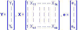
The actual computations involved in solving regression problems can be expressed compactly and conveniently using matrix notation. Suppose that there are n observed values of Y and n associated observed values for each of k different X variables. Then Yi, Xik, and ei can represent the ith observation of the Y variable, the ith observation of each of the X variables, and the ith unknown residual value, respectively. Collecting these terms into matrices we have
The multiple regression model in matrix notation then can be expressed as
Y = Xb + e where b is a column vector of 1 (for the intercept) + k unknown regression coefficients. Recall that the goal of multiple regression is to minimize the sum of the squared residuals. Regression coefficients that satisfy this criterion are found by solving the set of normal equations
X'Xb = X'Y When the X variables are linearly independent (i.e., they are nonredundant, yielding an X'X matrix which is of full rank) there is a unique solution to the normal equations. Premultiplying both sides of the matrix formula for the normal equations by the inverse of X'X gives
(X'X)-1X'Xb = (X'X)-1X'Y or
b = (X'X)-1X'Y
This last result is very satisfying in view of its simplicity and its generality. With regard to its simplicity, it expresses the solution for the regression equation in terms just 2 matrices (X and Y) and 3 basic matrix operations, (1) matrix transposition, which involves interchanging the elements in the rows and columns of a matrix, (2) matrix multiplication, which involves finding the sum of the products of the elements for each row and column combination of two conformable (i.e., multipliable) matrices, and (3) matrix inversion, which involves finding the matrix equivalent of a numeric reciprocal, that is, the matrix that satisfies
A-1AA=A
for a matrix A.
It took literally centuries for the ablest mathematicians and statisticians to find a satisfactory method for solving the linear least square regression problem. But their efforts have paid off, for it is hard to imagine a simpler solution.
With regard to the generality of the multiple regression model, its only notable limitations are that (1) it can be used to analyze only a single dependent variable, (2) it cannot provide a solution for the regression coefficients when the X variables are not linearly independent and the inverse of X'X therefore does not exist. These restrictions, however, can be overcome, and in doing so the multiple regression model is transformed into the general linear model.
| To index |
Extension of Multiple Regression to the General Linear Model
One way in which the general linear model differs from the multiple regression model is in terms of the number of dependent variables that can be analyzed. The Y vector of n observations of a single Y variable can be replaced by a Y matrix of n observations of m different Y variables. Similarly, the b vector of regression coefficients for a single Y variable can be replaced by a b matrix of regression coefficients, with one vector of b coefficients for each of the m dependent variables. These substitutions yield what is sometimes called the multivariate regression model, but it should be emphasized that the matrix formulations of the multiple and multivariate regression models are identical, except for the number of columns in the Y and b matrices. The method for solving for the b coefficients is also identical, that is, m different sets of regression coefficients are separately found for the m different dependent variables in the multivariate regression model.
The general linear model goes a step beyond the multivariate regression model by allowing for linear transformations or linear combinations of multiple dependent variables. This extension gives the general linear model important advantages over the multiple and the so-called multivariate regression models, both of which are inherently univariate (single dependent variable) methods. One advantage is that multivariate tests of significance can be employed when responses on multiple dependent variables are correlated. Separate univariate tests of significance for correlated dependent variables are not independent and may not be appropriate. Multivariate tests of significance of independent linear combinations of multiple dependent variables also can give insight into which dimensions of the response variables are, and are not, related to the predictor variables. Another advantage is the ability to analyze effects of repeated measure factors. Repeated measure designs, or within-subject designs, have traditionally been analyzed using ANOVA techniques. Linear combinations of responses reflecting a repeated measure effect (for example, the difference of responses on a measure under differing conditions) can be constructed and tested for significance using either the univariate or multivariate approach to analyzing repeated measures in the general linear model.
A second important way in which the general linear model differs from the multiple regression model is in its ability to provide a solution for the normal equations when the X variables are not linearly independent and the inverse of X'Xdoes not exist. Redundancy of the X variables may be incidental (e.g., two predictor variables might happen to be perfectly correlated in a small data set), accidental (e.g., two copies of the same variable might unintentionally be used in an analysis) or designed (e.g., indicator variables with exactly opposite values might be used in the analysis, as when both Male and Female predictor variables are used in representing Gender). Finding the regular inverse of a non-full-rank matrix is reminiscent of the problem of finding the reciprocal of 0 in ordinary arithmetic. No such inverse or reciprocal exists because division by 0 is not permitted. This problem is solved in the general linear model by using a generalized inverse of the X'X matrix in solving the normal equations. A generalized inverse is any matrix that satisfies
AA-A = A
for a matrix A.
A generalized inverse is unique and is the same as the regular inverse only if the matrix A is full rank. A generalized inverse for a non-full-rank matrix can be computed by the simple expedient of zeroing the elements in redundant rows and columns of the matrix. Suppose that an X'X matrix with r non-redundant columns is partitioned as
![]()
where A11 is an r by r matrix of rank r. Then the regular inverse of A11 exists and a generalized inverse of X'X is
![]()
where each 0 (null) matrix is a matrix of 0's (zeroes) and has the same dimensions as the corresponding A matrix.
In practice, however, a particular generalized inverse of X'X for finding a solution to the normal equations is usually computed using the sweep operator (Dempster, 1960). This generalized inverse, called a g2 inverse, has two important properties. One is that zeroing of the elements in redundant rows is unnecessary. Another is that partitioning or reordering of the columns of X'X is unnecessary, so that the matrix can be inverted "in place."
There are infinitely many generalized inverses of a non-full-rank X'X matrix, and thus, infinitely many solutions to the normal equations. This can make it difficult to understand the nature of the relationships of the predictor variables to responses on the dependent variables, because the regression coefficients can change depending on the particular generalized inverse chosen for solving the normal equations. It is not cause for dismay, however, because of the invariance properties of many results obtained using the general linear model.
A simple example may be useful for illustrating one of the most important invariance properties of the use of generalized inverses in the general linear model. If both Male and Female predictor variables with exactly opposite values are used in an analysis to represent Gender, it is essentially arbitrary as to which predictor variable is considered to be redundant (e.g., Male can be considered to be redundant with Female, or vice versa). No matter which predictor variable is considered to be redundant, no matter which corresponding generalized inverse is used in solving the normal equations, and no matter which resulting regression equation is used for computing predicted values on the dependent variables, the predicted values and the corresponding residuals for males and females will be unchanged. In using the general linear model, one must keep in mind that finding a particular arbitrary solution to the normal equations is primarily a means to the end of accounting for responses on the dependent variables, and not necessarily an end in itself.
| To index |
Sigma-Restricted and Overparameterized Model
Unlike the multiple regression model, which is usually applied to cases where the X variables are continuous, the general linear model is frequently applied to analyze any ANOVA or MANOVA design with categorical predictor variables, any ANCOVA or MANCOVA design with both categorical and continuous predictor variables, as well as any multiple or multivariate regression design with continuous predictor variables. To illustrate, Gender is clearly a nominal level variable (anyone who attempts to rank order the sexes on any dimension does so at his or her own peril in today's world). There are two basic methods by which Gender can be coded into one or more (non-offensive) predictor variables, and analyzed using the general linear model.
Sigma-restricted model (coding of categorical predictors). Using the first method, males and females can be assigned any two arbitrary, but distinct values on a single predictor variable. The values on the resulting predictor variable will represent a quantitative contrast between males and females. Typically, the values corresponding to group membership are chosen not arbitrarily but rather to facilitate interpretation of the regression coefficient associated with the predictor variable. In one widely used strategy, cases in the two groups are assigned values of 1 and -1 on the predictor variable, so that if the regression coefficient for the variable is positive, the group coded as 1 on the predictor variable will have a higher predicted value (i.e., a higher group mean) on the dependent variable, and if the regression coefficient is negative, the group coded as -1 on the predictor variable will have a higher predicted value on the dependent variable. An additional advantage is that since each group is coded with a value one unit from zero, this helps in interpreting the magnitude of differences in predicted values between groups, because regression coefficients reflect the units of change in the dependent variable for each unit change in the predictor variable. This coding strategy is aptly called the sigma-restricted parameterization, because the values used to represent group membership (1 and -1) sum to zero.
Note that the sigma-restricted parameterization of categorical predictor variables usually leads to X'X matrices which do not require a generalized inverse for solving the normal equations. Potentially redundant information, such as the characteristics of maleness and femaleness, is literally reduced to full-rank by creating quantitative contrast variables representing differences in characteristics.
Overparameterized model (coding of categorical predictors). The second basic method for recoding categorical predictorsr is the indicator variable approach. In this method a separate predictor variable is coded for each group identified by a categorical predictor variable. To illustrate, females might be assigned a value of 1 and males a value of 0 on a first predictor variable identifying membership in the female Gender group, and males would then be assigned a value of 1 and females a value of 0 on a second predictor variable identifying membership in the male Gender group. Note that this method of recoding categorical predictor variables will almost always lead to X'X matrices with redundant columns, and thus require a generalized inverse for solving the normal equations. As such, this method is often called the overparameterized model for representing categorical predictor variables, because it results in more columns in the X'X than are necessary for determining the relationships of categorical predictor variables to responses on the dependent variables.
True to its description as general, the general linear model can be used to perform analyses with categorical predictor variables which are coded using either of the two basic methods that have been described.
| To index |
To conclude this discussion of the ways in which the general linear model extends and generalizes regression methods, the general linear model can be expressed as
YM = Xb + e Here Y, X, b, and e are as described for the multivariate regression model and M is an m x s matrix of coefficients defining s linear transformation of the dependent variables. The normal equations are
X'Xb = X'YM and a solution for the normal equations is given by
b = (X'X)-X'YM Here the inverse of X'X is a generalized inverse if X'X contains redundant columns.
Add a provision for analyzing linear combinations of multiple dependent variables, add a method for dealing with redundant predictor variables and recoded categorical predictor variables, and the major limitations of multiple regression are overcome by the general linear model.
| To index |
A wide variety of types of designs can be analyzed using the general linear model. In fact, the flexibility of the general linear model allows it to handle so many different types of designs that it is difficult to develop simple typologies of the ways in which these designs might differ. Some general ways in which designs might differ can be suggested, but keep in mind that any particular design can be a "hybrid" in the sense that it could have combinations of features of a number of different types of designs.
In the following discussion, references will be made to the design matrix X, as well as sigma-restricted and overparameterized model coding. For an explanation of this terminology, refer to the secion entitled Basic Ideas: The General Linear Model, or, for a brief summary, to the Summary of computations section.
A basic discussion to univariate and multivariate ANOVA techniques can also be found in the ANOVA/MANOVA chapter; a discussion of mutiple regression methods is also provided in the Multiple Regression chapter.
Overview. The levels or values of the predictor variables in an analysis describe the differences between the n subjects or the n valid cases that are analyzed. Thus, when we speak of the between subject design (or simply the between design) for an analysis, we are referring to the nature, number, and arrangement of the predictor variables.
Concerning the nature or type of predictor variables, between designs which contain only categorical predictor variables can be called ANOVA (analysis of variance) designs, between designs which contain only continuous predictor variables can be called regression designs, and between designs which contain both categorical and continuous predictor variables can be called ANCOVA (analysis of covariance) designs. Further, continuous predictors are always considered to have fixed values, but the levels of categorical predictors can be considered to be fixed or to vary randomly. Designs which contain random categorical factors are called mixed-model designs (see the Variance Components and Mixed Model ANOVA/ANCOVA chapter).
Between designs may involve only a single predictor variable and therefore be described as simple (e.g., simple regression) or may employ numerous predictor variables (e.g., multiple regression).
Concerning the arrangement of predictor variables, some between designs employ only "main effect" or first-order terms for predictors, that is, the values for different predictor variables are independent and raised only to the first power. Other between designs may employ higher-order terms for predictors by raising the values for the original predictor variables to a power greater than 1 (e.g., in polynomial regression designs), or by forming products of different predictor variables (i.e., interaction terms). A common arrangement for ANOVA designs is the full-factorial design, in which every combination of levels for each of the categorical predictor variables is represented in the design. Designs with some but not all combinations of levels for each of the categorical predictor variables are aptly called fractional factorial designs. Designs with a hierarchy of combinations of levels for the different categorical predictor variables are called nested designs.
These basic distinctions about the nature, number, and arrangement of predictor variables can be used in describing a variety of different types of between designs. Some of the more common between designs can now be described.
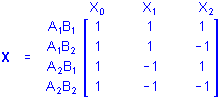
One-Way ANOVA. A design with a single categorical predictor variable is called a one-way ANOVA design. For example, a study of 4 different fertilizers used on different individual plants could be analyzed via one-way ANOVA, with four levels for the factor Fertilizer.
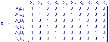
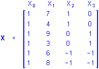
In genera, consider a single categorical predictor variable A with 1 case in each of its 3 categories. Using the sigma-restricted coding of A into 2 quantitative contrast variables, the matrix X defining the between design is
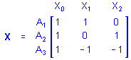
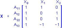
That is, cases in groups A1, A2, and A3 are all assigned values of 1 on X0 (the intercept), the case in group A1 is assigned a value of 1 on X1 and a value 0 on X2, the case in group A2 is assigned a value of 0 on X1 and a value 1 on X2, and the case in group A3 is assigned a value of -1 on X1 and a value -1 on X2. Of course, any additional cases in any of the 3 groups would be coded similarly. If there were 1 case in group A1, 2 cases in group A2, and 1 case in group A3, the X matrix would be
where the first subscript for A gives the replicate number for the cases in each group. For brevity, replicates usually are not shown when describing ANOVA design matrices.
Note that in one-way designs with an equal number of cases in each group, sigma-restricted coding yields X1 � Xk variables all of which have means of 0.
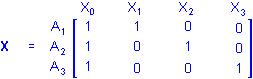
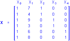
Using the overparameterized model to represent A, the X matrix defining the between design is simply
These simple examples show that the X matrix actually serves two purposes. It specifies (1) the coding for the levels of the original predictor variables on the X variables used in the analysis as well as (2) the nature, number, and arrangement of the X variables, that is, the between design.
Main Effect ANOVA. Main effect ANOVA designs contain separate one-way ANOVA designs for 2 or more categorical predictors. A good example of main effect ANOVA would be the typical analysis performed on screening designs as described in the context of the Experimental Design chapter.
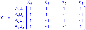
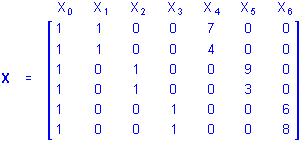
Consider 2 categorical predictor variables A and B each with 2 categories. Using the sigma-restricted coding, the X matrix defining the between design is
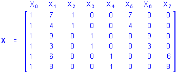
Note that if there are equal numbers of cases in each group, the sum of the cross-products of values for the X1 and X2 columns is 0, for example, with 1 case in each group (1*1)+(1*-1)+(-1*1)+(-1*-1)=0. Using the overparameterized model, the matrix X defining the between design is
Comparing the two types of coding, it can be seen that the overparameterized coding takes almost twice as many values as the sigma-restricted coding to convey the same information.
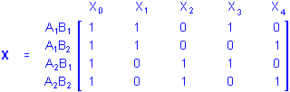
Factorial ANOVA. Factorial ANOVA designs contain X variables representing combinations of the levels of 2 or more categorical predictors (e.g., a study of boys and girls in four age groups, resulting in a 2 (Gender) x 4 (Age Group) design). In particular, full-factorial designs represent all possible combinations of the levels of the categorical predictors. A full-factorial design with 2 categorical predictor variables A and B each with 2 levels each would be called a 2 x 2 full-factorial design. Using the sigma-restricted coding, the X matrix for this design would be
Several features of this X matrix deserve comment. Note that the X1 and X2 columns represent main effect contrasts for one variable, (i.e., A and B, respectively) collapsing across the levels of the other variable. The X3 column instead represents a contrast between different combinations of the levels of A and B. Note also that the values for X3 are products of the corresponding values for X1 and X2. Product variables such as X3 represent the multiplicative or interaction effects of their factors, so X3 would be said to represent the 2-way interaction of A and B. The relationship of such product variables to the dependent variables indicate the interactive influences of the factors on responses above and beyond their independent (i.e., main effect) influences on responses. Thus, factorial designs provide more information about the relationships between categorical predictor variables and responses on the dependent variables than is provided by corresponding one-way or main effect designs.
When many factors are being investigated, however, full-factorial designs sometimes require more data than reasonably can be collected to represent all possible combinations of levels of the factors, and high-order interactions between many factors can become difficult to interpret. With many factors, a useful alternative to the full-factorial design is the fractional factorial design. As an example, consider a 2 x 2 x 2 fractional factorial design to degree 2 with 3 categorical predictor variables each with 2 levels. The design would include the main effects for each variable, and all 2-way interactions between the three variables, but would not include the 3-way interaction between all three variables. Using the overparameterized model, the X matrix for this design is
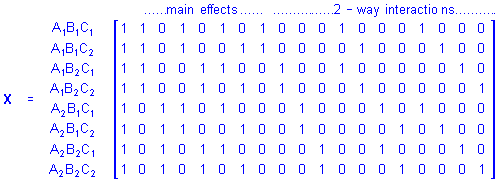
The 2-way interactions are the highest degree effects included in the design. These types of designs are discussed in detail the 2**(k-p) Fractional Factorial Designs section of the Experimental Design chapter.
Nested ANOVA Designs. Nested designs are similar to fractional factorial designs in that all possible combinations of the levels of the categorical predictor variables are not represented in the design. In nested designs, however, the omitted effects are lower-order effects. Nested effects are effects in which the nested variables never appear as main effects. Suppose that for 2 variables A and B with 3 and 2 levels, respectively, the design includes the main effect for A and the effect of B nested within the levels of A. The X matrix for this design using the overparameterized model is
Note that if the sigma-restricted coding were used, there would be only 2 columns in the X matrix for the B nested within A effect instead of the 6 columns in the X matrix for this effect when the overparameterized model coding is used (i.e., columns X4 through X9). The sigma-restricted coding method is overly-restrictive for nested designs, so only the overparameterized model is used to represent nested designs.
Balanced ANOVA. Most of the between designs discussed in this section can be analyzed much more efficiently, when they are balanced, i.e., when all cells in the ANOVA design have equal n, when there are no missing cells in the design, and, if nesting is present, when the nesting is balanced so that equal numbers of levels of the factors that are nested appear in the levels of the factor(s) that they are nested in. In that case, the X'X matrix (where X stands for the design matrix) is a diagonal matrix, and many of the computations necessary to compute the ANOVA results (such as matrix inversion) are greatly simplified.
Simple Regression. Simple regression designs involve a single continuous predictor variable. If there were 3 cases with values on a predictor variable P of, say, 7, 4, and 9, and the design is for the first-order effect of P, the X matrix would be
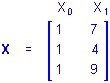
and using P for X1 the regression equation would be
Y = b0 + b1P
If the simple regression design is for a higher-order effect of P, say the quadratic effect, the values in the X1 column of the design matrix would be raised to the 2nd power, that is, squared
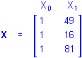
and using P2 for X1 the regression equation would be
Y = b0 + b1P2
The sigma-restricted and overparameterized coding methods do not apply to simple regression designs and any other design containing only continuous predictors (since there are no categorical predictors to code). Regardless of which coding method is chosen, values on the continuous predictor variables are raised to the desired power and used as the values for the X variables. No recoding is performed. It is therefore sufficient, in describing regression designs, to simply describe the regression equation without explicitly describing the design matrix X.
Multiple Regression. Multiple regression designs are to continuous predictor variables as main effect ANOVA designs are to categorical predictor variables, that is, multiple regression designs contain the separate simple regression designs for 2 or more continuous predictor variables. The regression equation for a multiple regression design for the first-order effects of 3 continuous predictor variables P, Q, and R would be
Y = b0 + b1P + b2Q + b3R
Factorial Regression. Factorial regression designs are similar to factorial ANOVA designs, in which combinations of the levels of the factors are represented in the design. In factorial regression designs, however, there may be many more such possible combinations of distinct levels for the continuous predictor variables than there are cases in the data set. To simplify matters, full-factorial regression designs are defined as designs in which all possible products of the continuous predictor variables are represented in the design. For example, the full-factorial regression design for two continuous predictor variables P and Q would include the main effects (i.e., the first-order effects) of P and Q and their 2-way P by Q interaction effect, which is represented by the product of P and Q scores for each case. The regression equation would be
Y = b0 + b1P + b2Q + b3P*Q
Factorial regression designs can also be fractional, that is, higher-order effects can be omitted from the design. A fractional factorial design to degree 2 for 3 continuous predictor variables P, Q, and R would include the main effects and all 2-way interactions between the predictor variables
Y = b0 + b1P + b2Q + b3R + b4P*Q + b5P*R + b6Q*R
Polynomial Regression. Polynomial regression designs are designs which contain main effects and higher-order effects for the continuous predictor variables but do not include interaction effects between predictor variables. For example, the polynomial regression design to degree 2 for three continuous predictor variables P, Q, and R would include the main effects (i.e., the first-order effects) of P, Q, and R and their quadratic (i.e., second-order) effects, but not the 2-way interaction effects or the P by Q by R 3-way interaction effect.
Y = b0 + b1P + b2P2 + b3Q + b4Q2 + b5R + b6R2
Polynomial regression designs do not have to contain all effects up to the same degree for every predictor variable. For example, main, quadratic, and cubic effects could be included in the design for some predictor variables, and effects up the fourth degree could be included in the design for other predictor variables.
Response Surface Regression. Quadratic response surface regression designs are a hybrid type of design with characteristics of both polynomial regression designs and fractional factorial regression designs. Quadratic response surface regression designs contain all the same effects of polynomial regression designs to degree 2 and additionally the 2-way interaction effects of the predictor variables. The regression equation for a quadratic response surface regression design for 3 continuous predictor variables P, Q, and R would be
Y = b0 + b1P + b2P2 + b3Q + b4Q2 + b5R + b6R2 + b7P*Q + b8P*R + b9Q*R
These types of designs are commonly employed in applied research (e.g., in industrial experimation), and a detailed discussion of these types of designs is also presented in the Experimental Design chapter (see Central composite designs).
Mixture Surface Regression. Mixture surface regression designs are identical to factorial regression designs to degree 2 except for the omission of the intercept. Mixtures, as the name implies, add up to a constant value; the sum of the proportions of ingredients in different recipes for some material all must add up 100%. Thus, the proportion of one ingredient in a material is redundant with the remaining ingredients. Mixture surface regression designs deal with this redundancy by omitting the intercept from the design. The design matrix for a mixture surface regression design for 3 continuous predictor variables P, Q, and R would be
Y = b1P + b2Q + b3R + b4P*Q + b5P*R + b6Q*R
These types of designs are commonly employed in applied research (e.g., in industrial experimation), and a detailed discussion of these types of designs is also presented in the Experimental Design chapter (see Mixture designs and triangular surfaces).
Analysis of Covariance. In general, between designs which contain both categorical and continuous predictor variables can be called ANCOVA designs. Traditionally, however, ANCOVA designs have referred more specifically to designs in which the first-order effects of one or more continuous predictor variables are taken into account when assessing the effects of one or more categorical predictor variables. A basic introduction to analysis of covariance can also be found in the Analysis of covariance (ANCOVA) topic of the ANOVA/MANOVA chapter.
To illustrate, suppose a researcher wants to assess the influences of a categorical predictor variable A with 3 levels on some outcome, and that measurements on a continuous predictor variable P, known to covary with the outcome, are available. If the data for the analysis are
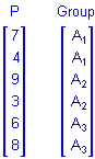
then the sigma-restricted X matrix for the design that includes the separate first-order effects of P and A would be
The b2 and b3 coefficients in the regression equation
Y = b0 + b1X1 + b2X2 + b3X3
represent the influences of group membership on the A categorical predictor variable, controlling for the influence of scores on the P continuous predictor variable. Similarly, the b1 coefficient represents the influence of scores on P controlling for the influences of group membership on A. This traditional ANCOVA analysis gives a more sensitive test of the influence of A to the extent that P reduces the prediction error, that is, the residuals for the outcome variable.
The X matrix for the same design using the overparameterized model would be
The interpretation is unchanged except that the influences of group membership on the A categorical predictor variables are represented by the b2, b3 and b4 coefficients in the regression equation
Y = b0 + b1X1 + b2X2 + b3X3 + b4X4
Separate Slope Designs. The traditional analysis of covariance (ANCOVA) design for categorical and continuous predictor variables is inappropriate when the categorical and continuous predictors interact in influencing responses on the outcome. The appropriate design for modeling the influences of the predictors in this situation is called the separate slope design. For the same example data used to illustrate traditional ANCOVA, the overparameterized X matrix for the design that includes the main effect of the three-level categorical predictor A and the 2-way interaction of P by A would be
The b4, b5, and b6 coefficients in the regression equation
Y = b0 + b1X1 + b2X2 + b3X3 + b4X4 + b5X5 + b6X6
give the separate slopes for the regression of the outcome on P within each group on A, controlling for the main effect of A.
As with nested ANOVA designs, the sigma-restricted coding of effects for separate slope designs is overly restrictive, so only the overparameterized model is used to represent separate slope designs. In fact, separate slope designs are identical in form to nested ANOVA designs, since the main effects for continuous predictors are omitted in separate slope designs.
Homogeneity of Slopes. The appropriate design for modeling the influences of continuous and categorical predictor variables depends on whether the continuous and categorical predictors interact in influencing the outcome. The traditional analysis of covariance (ANCOVA) design for continuous and categorical predictor variables is appropriate when the continuous and categorical predictors do not interact in influencing responses on the outcome, and the separate slope design is appropriate when the continuous and categorical predictors do interact in influencing responses. The homogeneity of slopes designs can be used to test whether the continuous and categorical predictors interact in influencing responses, and thus, whether the traditional ANCOVA design or the separate slope design is appropriate for modeling the effects of the predictors. For the same example data used to illustrate the traditional ANCOVA and separate slope designs, the overparameterized X matrix for the design that includes the main effect of P, the main effect of the three-level categorical predictor A, and the 2-way interaction of P by A would be
If the b5, b6, or b7 coefficient in the regression equation
Y = b0 + b1X1 + b2X2 + b3X3 + b4X4 + b5X5 + b6X6 + b7X7
is non-zero, the separate slope model should be used. If instead all 3 of these regression coefficients are zero the traditional ANCOVA design should be used.
The sigma-restricted X matrix for the homogeneity of slopes design would be
Using this X matrix, if the b4, or b5 coefficient in the regression equation
Y = b0 + b1X1 + b2X2 + b3X3 + b4X4 + b5X5
is non-zero, the separate slope model should be used. If instead both of these regression coefficients are zero the traditional ANCOVA design should be used.
Mixed Model ANOVA and ANCOVA. Designs which contain random effects for one or more categorical predictor variables are called mixed-model designs. Random effects are classification effects where the levels of the effects are assumed to be randomly selected from an infinite population of possible levels. The solution for the normal equations in mixed-model designs is identical to the solution for fixed-effect designs (i.e., designs which do not contain Random effects. Mixed-model designs differ from fixed-effect designs only in the way in which effects are tested for significance. In fixed-effect designs, between effects are always tested using the mean squared residual as the error term. In mixed-model designs, between effects are tested using relevant error terms based on the covariation of random sources of variation in the design. Specifically, this is done using Satterthwaite's method of denominator synthesis (Satterthwaite, 1946), which finds the linear combinations of sources of random variation that serve as appropriate error terms for testing the significance of the respective effect of interest. A basic discussion of these types of designs, and methods for estimating variance components for the random effects can also be found in the Variance Components and Mixed Model ANOVA/ANCOVA chapter.
Mixed-model designs, like nested designs and separate slope designs, are designs in which the sigma-restricted coding of categorical predictors is overly restrictive. Mixed-model designs require estimation of the covariation between the levels of categorical predictor variables, and the sigma-restricted coding of categorical predictors suppresses this covariation. Thus, only the overparameterized model is used to represent mixed-model designs (some programs will use the sigma-restricted approach and a so-called "restricted model" for random effects; however, only the overparameterized model as described in General Linear Models applies to both balanced and unbalanced designs, as well as designs with missing cells; see Searle, Casella, & McCullock, 1992, p. 127). It is important to recognize, however, that sigma-restricted coding can be used to represent any between design, with the exceptions of mixed-model, nested, and separate slope designs. Furthermore, some types of hypotheses can only be tested using the sigma-restricted coding (i.e., the effective hypothesis, Hocking, 1996), thus the greater generality of the overparameterized model for representing between designs does not justify it being used exclusively for representing categorical predictors in the general linear model.
| To index |
Within-Subject (Repeated Measures) Designs
Overview. It is quite common for researchers to administer the same test to the same subjects repeatedly over a period of time or under varying circumstances. In essence, one is interested in examining differences within each subject, for example, subjects' improvement over time. Such designs are referred to as within-subject designs or repeated measures designs. A basic introduction to repeated measures designs is also provided in the Between-groups and repeated measures topic of the ANOVA/MANOVA chapter.
For example, imagine that one wants to monitor the improvement of students' algebra skills over two months of instruction. A standardized algebra test is administered after one month (level 1 of the repeated measures factor), and a comparable test is administered after two months (level 2 of the repeated measures factor). Thus, the repeated measures factor (Time) has 2 levels.
Now, suppose that scores for the 2 algebra tests (i.e., values on the Y1 and Y2 variables at Time 1 and Time 2, respectively) are transformed into scores on a new composite variable (i.e., values on the T1), using the linear transformation
T = YM where M is an orthonormal contrast matrix. Specifically, if
then the difference of the mean score on T1 from 0 indicates the improvement (or deterioration) of scores across the 2 levels of Time.
One-Way Within-Subject Designs. The example algebra skills study with the Time repeated measures factor (see also within-subjects design Overview) illustrates a one-way within-subject design. In such designs, orthonormal contrast transformations of the scores on the original dependent Y variables are performed via the M transformation (orthonormal transformations correspond to orthogonal rotations of the original variable axes). If any b0 coefficient in the regression of a transformed T variable on the intercept is non-zero, this indicates a change in responses across the levels of the repeated measures factor, that is, the presence of a main effect for the repeated measure factor on responses.
What if the between design includes effects other than the intercept? If any of the b1 through bk coefficients in the regression of a transformed T variable on X are non-zero, this indicates a different change in responses across the levels of the repeated measures factor for different levels of the corresponding between effect, i.e., the presence of a within by between interaction effect on responses.
The same between-subject effects that can be tested in designs with no repeated-measures factors can also be tested in designs that do include repeated-measures factors. This is accomplished by creating a transformed dependent variable which is the sum of the original dependent variables divided by the square root of the number of original dependent variables. The same tests of between-subject effects that are performed in designs with no repeated-measures factors (including tests of the between intercept) are performed on this transformed dependent variable.
Multi-Way Within-Subject Designs. Suppose that in the example algebra skills study with the Time repeated measures factor (see the within-subject designs Overview), students were given a number problem test and then a word problem test on each testing occasion. Test could then be considered as a second repeated measures factor, with scores on the number problem tests representing responses at level 1 of the Test repeated measure factor, and scores on the word problem tests representing responses at level 2 of the Test repeated measure factor. The within subject design for the study would be a 2 (Time) by 2 (Test) full-factorial design, with effects for Time, Test, and the Time by Test interaction.
To construct transformed dependent variables representing the effects of Time, Test, and the Time by Test interaction, three respective M transformations of the original dependent Y variables are performed. Assuming that the original Y variables are in the order Time 1 - Test 1, Time 1 - Test 2, Time 2 - Test 1, and Time 2 - Test 2, the M matrices for the Time, Test, and the Time by Test interaction would be

The differences of the mean scores on the transformed T variables from 0 are then used to interpret the corresponding within-subject effects. If the b0 coefficient in the regression of a transformed T variable on the intercept is non-zero, this indicates a change in responses across the levels of a repeated measures effect, that is, the presence of the corresponding main or interaction effect for the repeated measure factors on responses.
Interpretation of within by between interaction effects follow the same procedures as for one-way within designs, except that now within by between interactions are examined for each within effect by between effect combination.
Multivariate Approach to Repeated Measures. When the repeated measures factor has more than 2 levels, then the M matrix will have more than a single column. For example, for a repeated measures factor with 3 levels (e.g., Time 1, Time 2, Time 3), the M matrix will have 2 columns (e.g., the two transformations of the dependent variables could be (1) Time 1 vs. Time 2 and Time 3 combined, and (2) Time 2 vs. Time 3). Consequently, the nature of the design is really multivariate, that is, there are two simultaneous dependent variables, which are transformations of the original dependent variables. Therefore, when testing repeated measures effects involving more than a single degree of freedom (e.g., a repeated measures main effect with more than 2 levels), you can compute multivariate test statistics to test the respective hypotheses. This is a different (and usually the preferred) approach than the univariate method that is still widely used. For a further discussion of the multivariate approach to testing repeated measures effects, and a comparison to the traditional univariate approach, see the Sphericity and compound symmetry topic of the ANOVA/MANOVA chapter.
Doubly Multivariate Designs. If the product of the number of levels for each within-subject factor is equal to the number of original dependent variables, the within-subject design is called a univariate repeated measures design. The within design is univariate because there is one dependent variable representing each combination of levels of the within-subject factors. Note that this use of the term univariate design is not to be confused with the univariate and multivariate approach to the analysis of repeated measures designs, both of which can be used to analyze such univariate (single-dependent-variable-only) designs. When there are two or more dependent variables for each combination of levels of the within-subject factors, the within-subject design is called a multivariate repeated measures design, or more commonly, a doubly multivariate within-subject design. This term is used because the analysis for each dependent measure can be done via the multivariate approach; so when there is more than one dependent measure, the design can be considered doubly-multivariate.
Doubly multivariate design are analyzed using a combination of univariate repeated measures and multivariate analysis techniques. To illustrate, suppose in an algebra skills study, tests are administered three times (repeated measures factor Time with 3 levels). Two test scores are recorded at each level of Time: a Number Problem score and a Word Problem score. Thus, scores on the two types of tests could be treated as multiple measures on which improvement (or deterioration) across Time could be assessed. M transformed variables could be computed for each set of test measures, and multivariate tests of significance could be performed on the multiple transformed measures, as well as on the each individual test measure.
Overview. When there are multiple dependent variables in a design, the design is said to be multivariate. Multivariate measures of association are by nature more complex than their univariate counterparts (such as the correlation coefficient, for example). This is because multivariate measures of association must take into account not only the relationships of the predictor variables with responses on the dependent variables, but also the relationships among the multiple dependent variables. By doing so, however, these measures of association provide information about the strength of the relationships between predictor and dependent variables independent of the dependent variable interrelationships. A basic discussion of multivariate designs is also presented in the Multivariate Designs topic in the ANOVA/MANOVA chapter.
The most commonly used multivariate measures of association all can be expressed as functions of the eigenvalues of the product matrix
E-1H
where E is the error SSCP matrix (i.e., the matrix of sums of squares and cross-products for the dependent variables that are not accounted for by the predictors in the between design), and H is a hypothesis SSCP matrix (i.e., the matrix of sums of squares and cross-products for the dependent variables that are accounted for by all the predictors in the between design, or the sums of squares and cross-products for the dependent variables that are accounted for by a particular effect). If
li = the ordered eigenvalues of E-1H, if E-1 exists
then the 4 commonly used multivariate measures of association are
Wilks' lambda = P[1/(1+li)]
Pillai's trace = Sli/(1+li)
Hotelling-Lawley trace = Sli
Roy's largest root = l1
These 4 measures have different upper and lower bounds, with Wilks' lambda perhaps being the most easily interpretable of the 4 measures. Wilks' lambda can range from 0 to 1, with 1 indicating no relationship of predictors to responses and 0 indicating a perfect relationship of predictors to responses. 1 - Wilks' lambda can be interpreted as the multivariate counterpart of a univariate R-squared, that is, it indicates the proportion of generalized variance in the dependent variables that is accounted for by the predictors.
The 4 measures of association are also used to construct multivariate tests of significance. These multivariate tests are covered in detail in a number of sources (e.g., Finn, 1974; Tatsuoka, 1971).
| To index |
Estimation and Hypothesis Testing
The following sections discuss details concerning hypothesis testing in the context of STATISTICA's VGLM module, for example, how the test for the overall model fit is computed, the options for computing tests for categorical effects in unbalanced or incomplete designs, how and when custom-error terms can be chosen, and the logic of testing custom-hypotheses in factorial or regression designs.
Partitioning Sums of Squares. A fundamental principle of least squares methods is that variation on a dependent variable can be partitioned, or divided into parts, according to the sources of the variation. Suppose that a dependent variable is regressed on one or more predictor variables, and that for covenience the dependent variable is scaled so that its mean is 0. Then a basic least squares identity is that the total sum of squared values on the dependent variable equals the sum of squared predicted values plus the sum of squared residual values. Stated more generally,
S(y - y-bar)2 = S(y-hat - y-bar)2 + S(y - y-hat)2
where the term on the left is the total sum of squared deviations of the observed values on the dependent variable from the dependent variable mean, and the respective terms on the right are (1) the sum of squared deviations of the predicted values for the dependent variable from the dependent variable mean and (2) the sum of the squared deviations of the observed values on the dependent variable from the predicted values, that is, the sum of the squared residuals. Stated yet another way,
Total SS = Model SS + Error SS
Note that the Total SS is always the same for any particular data set, but that the Model SS and the Error SS depend on the regression equation. Assuming again that the dependent variable is scaled so that its mean is 0, the Model SS and the Error SS can be computed using
Model SS = b'X'Y
Error SS = Y'Y - b'X'Y
Testing the Whole Model. Given the Model SS and the Error SS, one can perform a test that all the regression coefficients for the X variables (b1 through bk) are zero. This test is equivalent to a comparison of the fit of the regression surface defined by the predicted values (computed from the whole model regression equation) to the fit of the regression surface defined solely by the dependent variable mean (computed from the reduced regression equation containing only the intercept). Assuming that X'X is full-rank, the whole model hypothesis mean square
MSH = (Model SS)/k is an estimate of the variance of the predicted values. The error mean square
s2 = MSE = (Error SS)/(n-k-1)
is an unbiased estimate of the residual or error variance. The test statistic is
F = MSH/MSE
where F has (k, n - k - 1) degrees of freedom.
If X'X is not full rank, r + 1 is substituted for k, where r is the rank or the number of non-redundant columns of X'X.
Note that in the case of non-intercept models, some multiple regression programs will compute the full model test based on the proportion of variance around 0 (zero) accounted for by the predictors; for more information (see Kvålseth, 1985; Okunade, Chang, and Evans, 1993), while other will actually compute both values (i.e., based on the residual variance around 0, and around the respective dependent variable means.
Limitations of Whole Model Tests. For designs such as one-way ANOVA or simple regression designs, the whole model test by itself may be sufficient for testing general hypotheses about whether or not the single predictor variable is related to the outcome. In more complex designs, however, hypotheses about specific X variables or subsets of X variables are usually of interest. For example, one might want to make inferences about whether a subset of regression coefficients are 0, or one might want to test whether subpopulation means corresponding to combinations of specific X variables differ. The whole model test is usually insufficient for such purposes.
A variety of methods have been developed for testing specific hypotheses. Like whole model tests, many of these methods rely on comparisons of the fit of different models (e.g., Type I, Type II, and the effective hypothesis sums of squares). Other methods construct tests of linear combinations of regression coefficients in order to test mean differences (e.g., Type III, Type IV, and Type V sums of squares). For designs that contain only first-order effects of continuous predictor variables (i.e., multiple regression designs), many of these methods are equivalent (i.e., Type II through Type V sums of squares all test the significance of partial regression coefficients). However, there are important distinctions between the different hypothesis testing techniques for certain types of ANOVA designs (i.e., designs with unequal cell n's and/or missing cells).
All methods for testing hypotheses, however, involve the same hypothesis testing strategy employed in whole model tests, that is, the sums of squares attributable to an effect (using a given criterion) is computed, and then the mean square for the effect is tested using an appropriate error term.
| To index |
Six types of sums of squares
When there are categorical predictors in the model, arranged in a factorial ANOVA design, then one is typically interested in the main effects for and interaction effects between the categorical predictors. However, when the design is not balanced (has unequal cell n's, and consequently, the coded effects for the categorical factors are usually correlated), or when there are missing cells in a full factorial ANOVA design, then there is ambiguity regarding the specific comparisons between the (population, or least-squares) cell means that constitute the main effects and interactions of interest. These issues are discussed in great detail in Milliken and Johnson (1986), and if you routinely analyze incomplete factorial designs, you should consult their discussion of various problems and approaches to solving them.
In addition to the widely used methods that are commonly labeled Type I, II, III, and IV sums of squares (see Goodnight, 1980), we also offer different methods for testing effects in incomplete designs, that are widely used in other areas (and traditions) of research.
Type V sums of squares. Specifically, we propose the term Type V sums of squares to denote the approach that is widely used in industrial experimentation, to analyze fractional factorial designs; these types of designs are discussed in detail in the 2**(k-p) Fractional Factorial Designs section of the Experimental Design chapter. In effect, for those effects for which tests are performed all population marginal means (least squares means) are estimable.
Type VI sums of squares. Second, in keeping with the Type i labeling convention, we propose the term Type VI sums of squares to denote the approach that is often used in programs that only implement the sigma-restricted model (which is not well suited for certain types of designs; we offer a choice between the sigma-restricted and overparameterized model models). This approach is identical to what is described as the effective hypothesis method in Hocking (1996).
Contained Effects. The following descriptions will use the term contained effect. An effect E1 (e.g., A * B interaction) is contained in another effect E2 if:
Type I sums of squares are appropriate to use in balanced (equal n) ANOVA designs in which effects are entered into the model in their natural order (i.e., any main effects are entered before any two-way interaction effects, any two-way interaction effects are entered before any three-way interaction effects, and so on). Type I sums of squares are also useful in polynomial regression designs in which any lower-order effects are entered before any higher-order effects. A third use of Type I sums of squares is to test hypotheses for hierarchically nested designs, in which the first effect in the design is nested within the second effect, the second effect is nested within the third, and so on.
One important property of Type I sums of squares is that the sums of squares attributable to each effect add up to the whole model sums of squares. Thus, Type I sums of squares provide a complete decomposition of the predicted sums of squares for the whole model. This is not generally true for any other type of sums of squares. An important limitation of Type I sums of squares, however, is that the sums of squares attributable to a specific effect will generally depend on the order in which the effects are entered into the model. This lack of invariance to order of entry into the model limits the usefulness of Type I sums of squares for testing hypotheses for certain designs (e.g., fractional factorial designs).
Type II Sums of Squares. Type II sums of squares are sometimes called partially sequential sums of squares. Like Type I sums of squares, Type II sums of squares for an effect controls for the influence of other effects. Which other effects to control for, however, is determined by a different criterion. In Type II sums of squares, the sums of squares for an effect is computed by controlling for the influence of all other effects of equal or lower degree. Thus, sums of squares for main effects control for all other main effects, sums of squares for two-way interactions control for all main effects and all other two-way interactions, and so on.
Unlike Type I sums of squares, Type II sums of squares are invariant to the order in which effects are entered into the model. This makes Type II sums of squares useful for testing hypotheses for multiple regression designs, for main effect ANOVA designs, for full-factorial ANOVA designs with equal cell ns, and for hierarchically nested designs.
There is a drawback to the use of Type II sums of squares for factorial designs with unequal cell ns. In these situations, Type II sums of squares test hypotheses that are complex functions of the cell ns that ordinarily are not meaningful. Thus, a different method for testing hypotheses is usually preferred.
Type III Sums of Squares. Type I and Type II sums of squares usually are not appropriate for testing hypotheses for factorial ANOVA designs with unequal ns. For ANOVA designs with unequal ns, however, Type III sums of squares test the same hypothesis that would be tested if the cell ns were equal, provided that there is at least one observation in every cell. Specifically, in no-missing-cell designs, Type III sums of squares test hypotheses about differences in subpopulation (or marginal) means. When there are no missing cells in the design, these subpopulation means are least squares means, which are the best linear-unbiased estimates of the marginal means for the design (see, Milliken and Johnson, 1986).
Tests of differences in least squares means have the important property that they are invariant to the choice of the coding of effects for categorical predictor variables (e.g., the use of the sigma-restricted or overparameterized model) and to the choice of the particular g2 inverse of X'X used to solve the normal equations. Thus, tests of linear combinations of least squares means in general, including Type III tests of differences in least squares means, are said to not depend on the parameterization of the design. This makes Type III sums of squares useful for testing hypotheses for any design for which Type I or Type II sums of squares are appropriate, as well as for any unbalanced ANOVA design with no missing cells.
The Type III sums of squares attributable to an effect is computed as the sums of squares for the effect controlling for any effects of equal or lower degree and orthogonal to any higher-order interaction effects (if any) that contain it. The orthogonality to higher-order containing interactions is what gives Type III sums of squares the desirable properties associated with linear combinations of least squares means in ANOVA designs with no missing cells. But for ANOVA designs with missing cells, Type III sums of squares generally do not test hypotheses about least squares means, but instead test hypotheses that are complex functions of the patterns of missing cells in higher-order containing interactions and that are ordinarily not meaningful. In this situation Type V sums of squares or tests of the effective hypothesis (Type VI sums of squares) are preferred.
Type IV Sums of Squares. Type IV sums of squares were designed to test "balanced" hypotheses for lower-order effects in ANOVA designs with missing cells. Type IV sums of squares are computed by equitably distributing cell contrast coefficients for lower-order effects across the levels of higher-order containing interactions.
Type IV sums of squares are not recommended for testing hypotheses for lower-order effects in ANOVA designs with missing cells, even though this is the purpose for which they were developed. This is because Type IV sum-of-squares are invariant to some but not all g2 inverses of X'X that could be used to solve the normal equations. Specifically, Type IV sums of squares are invariant to the choice of a g2 inverse of X'X given a particular ordering of the levels of the categorical predictor variables, but are not invariant to different orderings of levels. Furthermore, as with Type III sums of squares, Type IV sums of squares test hypotheses that are complex functions of the patterns of missing cells in higher-order containing interactions and that are ordinarily not meaningful.
Statisticians who have examined the usefulness of Type IV sums of squares have concluded that Type IV sums of squares are not up to the task for which they were developed:
Type V Sums of Squares. Type V sums of squares were developed as an alternative to Type IV sums of squares for testing hypotheses in ANOVA designs in missing cells. Also, this approach is widely used in industrial experimentation, to analyze fractional factorial designs; these types of designs are discussed in detail in the 2**(k-p) Fractional Factorial Designs section of the Experimental Design chapter. In effect, for effects for which tests are performed all population marginal means (least squares means) are estimable.
Type V sums of squares involve a combination of the methods employed in computing Type I and Type III sums of squares. Specifically, whether or not an effect is eligible to be dropped from the model is determined using Type I procedures, and then hypotheses are tested for effects not dropped from the model using Type III procedures. Type V sums of squares can be illustrated by using a simple example. Suppose that the effects considered are A, B, and A by B, in that order, and that A and B are both categorical predictors with, say, 3 and 2 levels, respectively. The intercept is first entered into the model. Then A is entered into the model, and its degrees of freedom are determined (i.e., the number of non-redundant columns for A in X'X, given the intercept). If A's degrees of freedom are less than 2 (i.e., its number of levels minus 1), it is eligible to be dropped. Then B is entered into the model, and its degrees of freedom are determined (i.e., the number of non-redundant columns for B in X'X, given the intercept and A). If B's degrees of freedom are less than 1 (i.e., its number of levels minus 1), it is eligible to be dropped. Finally, A by B is entered into the model, and its degrees of freedom are determined (i.e., the number of non-redundant columns for A by B in X'X, given the intercept, A, and B). If B's degrees of freedom are less than 2 (i.e., the product of the degrees of freedom for its factors if there were no missing cells), it is eligible to be dropped. Type III sums of squares are then computed for the effects that were not found to be eligible to be dropped, using the reduced model in which any eligible effects are dropped. Tests of significance, however, use the error term for the whole model prior to dropping any eligible effects.
Note that Type V sums of squares involve determining a reduced model for which all effects remaining in the model have at least as many degrees of freedom as they would have if there were no missing cells. This is equivalent to finding a subdesign with no missing cells such that the Type III sums of squares for all effects in the subdesign reflect differences in least squares means.
Appropriate caution should be exercised when using Type V sums of squares. Dropping an effect from a model is the same as assuming that the effect is unrelated to the outcome (see, e.g., Hocking, 1996). The reasonableness of the assumption does not necessarily insure its validity, so when possible the relationships of dropped effects to the outcome should be inspected. It is also important to note that Type V sums of squares are not invariant to the order in which eligibility for dropping effects from the model is evaluated. Different orders of effects could produce different reduced models.
In spite of these limitations, Type V sums of squares for the reduced model have all the same properties of Type III sums of squares for ANOVA designs with no missing cells. Even in designs with many missing cells (such as fractional factorial designs, in which many high-order interaction effects are assumed to be zero), Type V sums of squares provide tests of meaningful hypotheses, and sometimes hypotheses that cannot be tested using any other method.
Type VI (Effective Hypothesis) Sums of Squares. Type I through Type V sums of squares can all be viewed as providing tests of hypotheses that subsets of partial regression coefficients (controlling for or orthogonal to appropriate additional effects) are zero. Effective hypothesis tests (developed by Hocking, 1996) are based on the philosophy that the only unambiguous estimate of an effect is the proportion of variability on the outcome that is uniquely attributable to the effect. The overparameterized coding of effects for categorical predictor variables generally cannot be used to provide such unique estimates for lower-order effects. Effective hypothesis tests, which we propose to call Type VI sums of squares, use the sigma-restricted coding of effects for categorical predictor variables to provide unique effect estimates even for lower-order effects.
The method for computing Type VI sums of squares is straightforward. The sigma-restricted coding of effects is used, and for each effect, its Type VI sums of squares is the difference of the model sums of squares for all other effects from the whole model sums of squares. As such, the Type VI sums of squares provide an unambiguous estimate of the variability of predicted values for the outcome uniquely attributable to each effect.
In ANOVA designs with missing cells, Type VI sums of squares for effects can have fewer degrees of freedom than they would have if there were no missing cells, and for some missing cell designs, can even have zero degrees of freedom. The philosophy of Type VI sums of squares is to test as much as possible of the original hypothesis given the observed cells. If the pattern of missing cells is such that no part of the original hypothesis can be tested, so be it. The inability to test hypotheses is simply the price one pays for having no observations at some combinations of the levels of the categorical predictor variables. The philosophy is that it is better to admit that a hypothesis cannot be tested than it is to test a distorted hypothesis which may not meaningfully reflect the original hypothesis.
Type VI sums of squares cannot generally be used to test hypotheses for nested ANOVA designs, separate slope designs, or mixed-model designs, because the sigma-restricted coding of effects for categorical predictor variables is overly restrictive in such designs. This limitation, however, does not diminish the fact that Type VI sums of squares can b
| To index |
Lack-of-Fit Tests using Pure Error. Whole model tests and tests based on the 6 types of sums of squares use the mean square residual as the error term for tests of significance. For certain types of designs, however, the residual sum of squares can be further partitioned into meaningful parts which are relevant for testing hypotheses. One such type of design is a simple regression design in which there are subsets of cases all having the same values on the predictor variable. For example, performance on a task could be measured for subjects who work on the task under several different room temperature conditions. The test of significance for the Temperature effect in the linear regression of Performance on Temperature would not necessarily provide complete information on how Temperature relates to Performance; the regression coefficient for Temperature only reflects its linear effect on the outcome.
One way to glean additional information from this type of design is to partition the residual sums of squares into lack-of-fit and pure error components. In the example just described, this would involve determining the difference between the sum of squares that cannot be predicted by Temperature levels, given the linear effect of Temperature (residual sums of squares) and the pure error; this difference would be the sums of squares associated with the lack-of-fit (in this example, of the linear model). The test of lack-of-fit, using the mean square pure error as the error term, would indicate whether non-linear effects of Temperature are needed to adequately model Tempature's influence on the outcome. Further, the linear effect could be tested using the pure error term, thus providing a more sensitive test of the linear effect independent of any possible nonlinear effect.
Designs with Zero Degrees of Freedom for Error. When the model degrees of freedom equal the number of cases or subjects, the residual sums of squares will have zero degrees of freedom and preclude the use of standard hypothesis tests. This sometimes occurs for overfitted designs (designs with many predictors, or designs with categorical predictors having many levels). However, in some designed experiments, such as experiments using split-plot designs or highly fractionalized factorial designs as commonly used in industrial experimentation, it is no accident that the residual sum of squares has zero degrees of freedom. In such experiments, mean squares for certain effects are planned to be used as error terms for testing other effects, and the experiment is designed with this in mind. It is entirely appropriate to use alternatives to the mean square residual as error terms for testing hypotheses in such designs.
Tests in Mixed Model Designs. Designs which contain random effects for one or more categorical predictor variables are called mixed-model designs. These types of designs, and the analysis of those designs, is also described in detail in the Variance Components and Mixed Model ANOVA/ANCOVA chapter. Random effects are classification effects where the levels of the effects are assumed to be randomly selected from an infinite population of possible levels. The solution for the normal equations in mixed-model designs is identical to the solution for fixed-effect designs (i.e., designs which do not contain random effects). Mixed-model designs differ from fixed-effect designs only in the way in which effects are tested for significance. In fixed-effect designs, between effects are always tested using the mean square residual as the error term. In mixed-model designs, between effects are tested using relevant error terms based on the covariation of sources of variation in the design. Also, only the overparameterized model is used to code effects for categorical predictors in mixed-models, because the sigma-restricted model is overly restrictive.
The covariation of sources of variation in the design is estimated by the elements of a matrix called the Expected Mean Squares (EMS) matrix. This non-square matrix contains elements for the covariation of each combination of pairs of sources of variation and for each source of variation with Error. Specifically, each element is the mean square for one effect (indicated by the column) that is expected to be accounted by another effect (indicated by the row), given the observed covariation in their levels. Note that expected mean squares can be computing using any type of sums of squares from Type I through Type V. Once the EMS matrix is computed, it is used to the solve for the linear combinations of sources of random variation that are appropriate to use as error terms for testing the significance of the respective effects. This is done using Satterthwaite's method of denominator synthesis (Satterthwaite, 1946). Detailed discussions of methods for testing effects in mixed-models, and related methods for estimating variance components for random effects, can be found in the Variance Components and Mixed Model ANOVA/ANCOVA chapter.
| To index |
Whole model tests and tests based on sums of squares attributable to specific effects illustrate two general types of hypotheses that can be tested using the general linear model. Still, there may be other types of hypotheses the researcher wishes to test that do not fall into either of these categories. For example, hypotheses about subsets of effects may be of interest, or hypotheses involving comparisons of specific levels of categorical predictor variables may be of interest.
Estimability of Hypotheses. Before considering tests of specific hypotheses of this sort, it is important to address the issue of estimability. A test of a specific hypothesis using the general linear model must be framed in terms of the regression coefficients for the solution of the normal equations. If the X'X matrix is less than full rank, the regression coefficients depend on the particular g2 inverse used for solving the normal equations, and the regression coefficients will not be unique. When the regression coefficients are not unique, linear functions (f) of the regression coefficients having the form
f = Lb
where L is a vector of coefficients, will also in general not be unique. However, Lb for an L which satisfies
L = L(X'X)-X'X
is invariant for all possible g2 inverses, and is therefore called an estimable function.
The theory of estimability of linear functions is an advanced topic in the theory of algebraic invariants (Searle, 1987, provides a comprehensive introduction), but its implications are clear enough. One instance of non-estimability of a hypothesis has been encountered in tests of the effective hypothesis which have zero degrees of freedom. On the other hand, Type III sums of squares for categorical predictor variable effects in ANOVA designs with no missing cells (and the least squares means in such designs) provide an example of estimable functions which do not depend on the model parameterization (i.e., the particular g2 inverse used to solve the normal equations). The general implication of the theory of estimability of linear functions is that hypotheses which cannot be expressed as linear combinations of the rows of X (i.e., the combinations of observed levels of the categorical predictor variables) are not estimable, and therefore cannot be tested. Stated another way, we simply cannot test specific hypotheses that are not represented in the data. The notion of estimability is valuable because the test for estimability makes explicit which specific hypotheses can be tested and which cannot.
Linear Combinations of Effects. In multiple regression designs, it is common for hypotheses of interest to involve subsets of effects. In mixture designs, for example, one might be interested in simultaneously testing whether the main effect and any of the two-way interactions involving a particular predictor variable are non-zero. It is also common in multiple regression designs for hypotheses of interest to involves comparison of slopes. For example, one might be interested in whether the regression coefficients for two predictor variables differ. In both factorial regression and factorial ANOVA designs with many factors, it is often of interest whether sets of effects, say, all three-way and higher-order interactions, are nonzero.
Tests of these types of specific hypotheses involve (1) constructing one or more Ls reflecting the hypothesis, (2) testing the estimability of the hypothesis by determining whether
L = L(X'X)-X'X
and if so, using (3)
(Lb)'
to estimate the sums of squares accounted for by the hypothesis. Finally, (4) the hypothesis is tested for significance using the usual mean square residual as the error term. To illustrate this 4-step procedure, suppose that a test of the difference in the regression slopes is desired for the (intercept plus) 2 predictor variables in a first-order multiple regression design. The coefficients for L would be
L = [0 1 -1]
(note that the first coefficient 0 excludes the intercept from the comparison) for which Lb is estimable if the 2 predictor variables are not redundant with each other. The hypothesis sums of squares reflect the difference in the partial regression coefficients for the 2 predictor variables, which is tested for significance using the mean square residual as the error term.
Planned Comparisons of Least Square Means. Usually, experimental hypotheses are stated in terms that are more specific than simply main effects or interactions. We may have the specific hypothesis that a particular textbook will improve math skills in males, but not in females, while another book would be about equally effective for both genders, but less effective overall for males. Now generally, we are predicting an interaction here: the effectiveness of the book is modified (qualified) by the student's gender. However, we have a particular prediction concerning the nature of the interaction: we expect a significant difference between genders for one book, but not the other. This type of specific prediction is usually tested by testing planned comparisons of least squares means (estimates of the population marginal means), or as it is sometimes called, contrast analysis.
Briefly, contrast analysis allows us to test the statistical significance of predicted specific differences in particular parts of our complex design. The 4-step procedure for testing specific hypotheses is used to specify and test specific predictions. Contrast analysis is a major and indispensable component of the analysis of many complex experimental designs (see also for details).
To learn more about the logic and interpretation of contrast analysis refer to the ANOVA/MANOVA chapter Overview section.
Post-Hoc Comparisons. Sometimes we find effects in an experiment that were not expected. Even though in most cases a creative experimenter will be able to explain almost any pattern of means, it would not be appropriate to analyze and evaluate that pattern as if one had predicted it all along. The problem here is one of capitalizing on chance when performing multiple tests post-hoc, that is, without a priori hypotheses. To illustrate this point, let us consider the following "experiment." Imagine we were to write down a number between 1 and 10 on 100 pieces of paper. We then put all of those pieces into a hat and draw 20 samples (of pieces of paper) of 5 observations each, and compute the means (from the numbers written on the pieces of paper) for each group. How likely do you think it is that we will find two sample means that are significantly different from each other? It is very likely! Selecting the extreme means obtained from 20 samples is very different from taking only 2 samples from the hat in the first place, which is what the test via the contrast analysis implies. Without going into further detail, there are several so-called post-hoc tests that are explicitly based on the first scenario (taking the extremes from 20 samples), that is, they are based on the assumption that we have chosen for our comparison the most extreme (different) means out of k total means in the design. Those tests apply "corrections" that are designed to offset the advantage of post-hoc selection of the most extreme comparisons. Whenever one finds unexpected results in an experiment one should use those post-hoc procedures to test their statistical significance.
| To index |
Testing hypotheses for repeated measures and dependent variables
In the discussion of different hypotheses that can be tested using the general linear model, the tests have been described as tests for "the dependent variable" or "the outcome." This has been done solely to simplify the discussion. When there are multiple dependent variables reflecting the levels of repeated measure factors, the general linear model performs tests using orthonormalized M-transformations of the dependent variables. When there are multiple dependent variables but no repeated measure factors, the general linear model performs tests using the hypothesis sums of squares and cross-products for the multiple dependent variables, which are tested against the residual sums of squares and cross-products for the multiple dependent variables. Thus, the same hypothesis testing procedures which apply to univariate designs with a single dependent variable also apply to repeated measure and multivariate designs.
| To index |
