Experiments in Science and Industry
Experimental methods are widely used in research as well as in industrial settings, however, sometimes for very different purposes. The primary goal in scientific research is usually to show the statistical significance of an effect that a particular factor exerts on the dependent variable of interest (for details concerning the concept of statistical significance see Elementary Concepts).
In industrial settings, the primary goal is usually to extract the maximum amount of unbiased information regarding the factors affecting a production process from as few (costly) observations as possible. While in the former application (in science) analysis of variance (ANOVA) techniques are used to uncover the interactive nature of reality, as manifested in higher-order interactions of factors, in indus"nuisance" (they are often of no interest; they only complicate the process of identifying important factors).
Differences in techniques
These differences in purpose have a profound effect on the techniques that are used in the two settings. If you review a standard ANOVA text for the sciences, for example the classic texts by Winer (1962) or Keppel (1982), you will find that they will primarily discuss designs with up to, perhaps, five factors (designs with more than six factors are usually impractical; see the ANOVA/MANOVA chapter). The focus of these discussions is how to derive valid and robust statistical significance tests. However, if you review standard texts on experimentation in industry (Box, Hunter, and Hunter, 1978; Box and Draper, 1987; Mason, Gunst, and Hess, 1989; Taguchi, 1987) you will find that they will primarily discuss designs with many factors (e.g., 16 or 32) in which interaction effects cannot be evaluated, and the primary focus of the discussion is how to derive unbiased main effect (and, perhaps, two-way interaction) estimates with a minimum number of observations.
This comparison can be expanded further, however, a more detailed description of experimental design in industry will now be discussed and other differences will become clear. Note that the General Linear Models and ANOVA/MANOVA chapters contain detailed discussions of typical design issues in scientific research; the General Linear Model procedure is a very comprehensive implementation of the general linear model approach to ANOVA/MANOVA (univariate and multivariate ANOVA). There are of course applications in industry where general ANOVA designs, as used in scientific research, can be immensely useful. You may want to read the General Linear Models and ANOVA/MANOVA chapters to gain a more general appreciation of the range of methods encompassed by the term Experimental Design.
Overview
The general ideas and principles on which experimentation in industry is based, and the types of designs used will be discussed in the following paragraphs. The following paragraphs are meant to be introductory in nature. However, it is assumed that you are familiar with the basic ideas of analysis of variance and the interpretation of main effects and interactions in ANOVA. Otherwise, it is strongly recommend that you read the Introductory Overview section for ANOVA/MANOVA and the General Linear Models chapter.
General Ideas
In general, every machine used in a production process allows its operators to adjust various settings, affecting the resultant quality of the product manufactured by the machine. Experimentation allows the production engineer to adjust the settings of the machine in a systematic manner and to learn which factors have the greatest impact on the resultant quality. Using this information, the settings can be constantly improved until optimum quality is obtained. To illustrate this reasoning, here are a few examples:
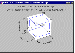
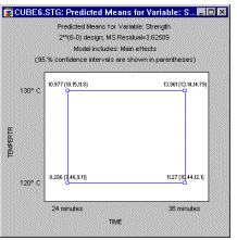
Example 1: Dyestuff manufacture. Box and Draper (1987, page 115) report an experiment concerned with the manufacture of certain dyestuff. Quality in this context can be described in terms of a desired (specified) hue and brightness and maximum fabric strength. Moreover, it is important to know what to change in order to produce a different hue and brightness should the consumers' taste change. Put another way, the experimenter would like to identify the factors that affect the brightness, hue, and strength of the final product. In the example described by Box and Draper, there are 6 different factors that are evaluated in a 2**(6-0) design (the 2**(k-p) notation is explained below). The results of the experiment show that the three most important factors determining fabric strength are the Polysulfide index, Time, and Temperature (see Box and Draper, 1987, page 116). One can summarize the expected effect (predicted means) for the variable of interest (i.e., fabric strength in this case) in a so- called cube-plot. This plot shows the expected (predicted) mean fabric strength for the respective low and high settings for each of the three variables (factors).

Example 1.1: Screening designs. In the previous example, 6 different factors were simultaneously evaluated. It is not uncommon, that there are very many (e.g., 100) different factors that may potentially be important. Special designs (e.g., Plackett-Burman designs, see Plackett and Burman, 1946) have been developed to screen such large numbers of factors in an efficient manner, that is, with the least number of observations necessary. For example, you can design and analyze an experiment with 127 factors and only 128 runs (observations); still, you will be able to estimate the main effects for each factor, and thus, you can quickly identify which ones are important and most likely to yield improvements in the process under study.
Example 2: 3**3 design. Montgomery (1976, page 204) describes an experiment conducted in order identify the factors that contribute to the loss of soft drink syrup due to frothing during the filling of five- gallon metal containers. Three factors where considered: (a) the nozzle configuration, (b) the operator of the machine, and (c) the operating pressure. Each factor was set at three different levels, resulting in a complete 3**(3-0) experimental design (the 3**(k-p) notation is explained below).
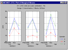
Moreover, two measurements were taken for each combination of factor settings, that is, the 3**(3-0) design was completely replicated once.
Example 3: Maximizing yield of a chemical reaction. The yield of many chemical reactions is a function of time and temperature. Unfortunately, these two variables often do not affect the resultant yield in a linear fashion. In other words, it is not so that "the longer the time, the greater the yield" and "the higher the temperature, the greater the yield." Rather, both of these variables are usually related in a curvilinear fashion to the resultant yield.
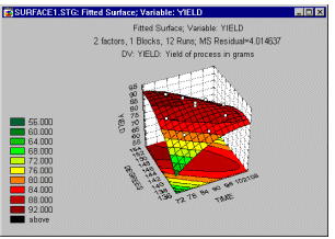
Thus, in this example your goal as experimenter would be to optimize the yield surface that is created by the two variables: time and temperature.
Example 4: Testing the effectiveness of four fuel additives. Latin square designs are useful when the factors of interest are measured at more than two levels, and the nature of the problem suggests some blocking. For example, imagine a study of 4 fuel additives on the reduction in oxides of nitrogen (see Box, Hunter, and Hunter, 1978, page 263). You may have 4 drivers and 4 cars at your disposal. You are not particularly interested in any effects of particular cars or drivers on the resultant oxide reduction; however, you do not want the results for the fuel additives to be biased by the particular driver or car. Latin square designs allow you to estimate the main effects of all factors in the design in an unbiased manner. With regard to the example, the arrangement of treatment levels in a Latin square design assures that the variability among drivers or cars does not affect the estimation of the effect due to different fuel additives.
Example 5: Improving surface uniformity in the manufacture of polysilicon wafers. The manufacture of reliable microprocessors requires very high consistency in the manufacturing process. Note that in this instance, it is equally, if not more important to control the variability of certain product characteristics than it is to control the average for a characteristic. For example, with regard to the average surface thickness of the polysilicon layer, the manufacturing process may be perfectly under control; yet, if the variability of the surface thickness on a wafer fluctuates widely, the resultant microchips will not be reliable. Phadke (1989) describes how different characteristics of the manufacturing process (such as deposition temperature, deposition pressure, nitrogen flow, etc.) affect the variability of the polysilicon surface thickness on wafers. However, no theoretical model exists that would allow the engineer to predict how these factors affect the uniformness of wafers. Therefore, systematic experimentation with the factors is required to optimize the process. This is a typical example where Taguchi robust design methods would be applied.
Example 6: Mixture designs. Cornell (1990, page 9) reports an example of a typical (simple) mixture problem. Specifically, a study was conducted to determine the optimum texture of fish patties as a result of the relative proportions of different types of fish (Mullet, Sheepshead, and Croaker) that made up the patties. Unlike in non-mixture experiments, the total sum of the proportions must be equal to a constant, for example, to 100%. The results of such experiments are usually graphically represented in so-called triangular (or ternary) graphs.
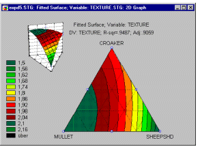
In general, the overall constraint -- that the three components must sum to a constant -- is reflected in the triangular shape of the graph (see above).
Example 6.1: Constrained mixture designs. It is particularly common in mixture designs that the relative amounts of components are further constrained (in addition to the constraint that they must sum to, for example, 100%). For example, suppose we wanted to design the best-tasting fruit punch consisting of a mixture of juices from five fruits. Since the resulting mixture is supposed to be a fruit punch, pure blends consisting of the pure juice of only one fruit are necessarily excluded. Additional constraints may be placed on the "universe" of mixtures due to cost constraints or other considerations, so that one particular fruit cannot, for example, account for more than 30% of the mixtures (otherwise the fruit punch would be too expensive, the shelf-life would be compromised, the punch could not be produced in large enough quantities, etc.). Such so-called constrained experimental regions present numerous problems, which, however, can be addressed.
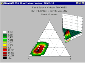
In general, under those conditions, one seeks to design an experiment that can potentially extract the maximum amount of information about the respective response function (e.g., taste of the fruit punch) in the experimental region of interest.
Computational Problems
There are basically two general issues to which Experimental Design is addressed:
Components of Variance, Denominator Synthesis
There are several statistical methods for analyzing designs with random effects (see Methods for Analysis of Variance). The Variance Components and Mixed Model ANOVA/ANCOVA chapter discusses numerous options for estimating variance components for random effects, and for performing approximate F tests based on synthesized error terms.
Summary
Experimental methods are finding increasing use in manufacturing to optimize the production process. Specifically, the goal of these methods is to identify the optimum settings for the different factors that affect the production process. In the discussion so far, the major classes of designs that are typically used in industrial experimentation have been introduced: 2**(k-p) (two-level, multi-factor) designs, screening designs for large numbers of factors, 3**(k-p) (three-level, multi-factor) designs (mixed designs with 2 and 3 level factors are also supported), central composite (or response surface) designs, Latin square designs, Taguchi robust design analysis, mixture designs, and special procedures for constructing experiments in constrained experimental regions. Interestingly, many of these experimental techniques have "made their way" from the production plant into management, and successful implementations have been reported in profit planning in business, cash-flow optimization in banking, etc. (e.g., see Yokyama and Taguchi, 1975).
These techniques will now be described in greater detail in the following sections:
In many cases, it is sufficient to consider the factors affecting the production process at two levels. For example, the temperature for a chemical process may either be set a little higher or a little lower, the amount of solvent in a dyestuff manufacturing process can either be slightly increased or decreased, etc. The experimenter would like to determine whether any of these changes affect the results of the production process. The most intuitive approach to study those factors would be to vary the factors of interest in a full factorial design, that is, to try all possible combinations of settings. This would work fine, except that the number of necessary runs in the experiment (observations) will increase geometrically. For example, if you want to study 7 factors, the necessary number of runs in the experiment would be 2**7 = 128. To study 10 factors you would need 2**10 = 1,024 runs in the experiment. Because each run may require time-consuming and costly setting and resetting of machinery, it is often not feasible to require that many different production runs for the experiment. In these conditions, fractional factorials are used that "sacrifice" interaction effects so that main effects may still be computed correctly.
Generating the Design
A technical description of how fractional factorial designs are constructed is beyond the scope of this introduction. Detailed accounts of how to design 2**(k-p) experiments can be found, for example, in Bayne and Rubin (1986), Box and Draper (1987), Box, Hunter, and Hunter (1978), Montgomery (1991), Daniel (1976), Deming and Morgan (1993), Mason, Gunst, and Hess (1989), or Ryan (1989), to name only a few of the many text books on this subject. In general, it will successively "use" the highest-order interactions to generate new factors. For example, consider the following design that includes 11 factors but requires only 16 runs (observations).
| Design: 2**(11-7), Resolution III | |||||||||||
|---|---|---|---|---|---|---|---|---|---|---|---|
| Run | A | B | C | D | E | F | G | H | I | J | K |
| 1 2 3 4 5 6 7 8 9 10 11 12 13 14 15 16 |
1 1 1 1 1 1 1 1 -1 -1 -1 -1 -1 -1 -1 -1 |
1 1 1 1 -1 -1 -1 -1 1 1 1 1 -1 -1 -1 -1 |
1 1 -1 -1 1 1 -1 -1 1 1 -1 -1 1 1 -1 -1 |
1 -1 1 -1 1 -1 1 -1 1 -1 1 -1 1 -1 1 -1 |
1 1 -1 -1 -1 -1 1 1 -1 -1 1 1 1 1 -1 -1 |
1 -1 -1 1 -1 1 1 -1 1 -1 -1 1 -1 1 1 -1 |
1 -1 -1 1 1 -1 -1 1 -1 1 1 -1 -1 1 1 -1 |
1 -1 1 -1 -1 1 -1 1 -1 1 -1 1 1 -1 1 -1 |
1 -1 -1 1 -1 1 1 -1 -1 1 1 -1 1 -1 -1 1 |
1 1 1 1 -1 -1 -1 -1 -1 -1 -1 -1 1 1 1 1 |
1 1 -1 -1 1 1 -1 -1 -1 -1 1 1 -1 -1 1 1 |
Reading the design. The design displayed above should be interpreted as follows. Each column contains +1's or -1's to indicate the setting of the respective factor (high or low, respectively). So for example, in the first run of the experiment, set all factors A through K to the plus setting (e.g., a little higher than before); in the second run, set factors A, B, and C to the positive setting, factor D to the negative setting, and so on. Note that there are numerous options provided to display (and save) the design using notation other than �1 to denote factor settings. For example, you may use actual values of factors (e.g., 90 degrees Celsius and 100 degrees Celsius) or text labels (Low temperature, High temperature).
Randomizing the runs. Because many other things may change from production run to production run, it is always a good practice to randomize the order in which the systematic runs of the designs are performed.
The Concept of Design Resolution
The design above is described as a 2**(11-7) design of resolution III (three). This means that you study overall k = 11 factors (the first number in parentheses); however, p = 7 of those factors (the second number in parentheses) were generated from the interactions of a full 2**[(11-7) = 4] factorial design. As a result, the design does not give full resolution; that is, there are certain interaction effects that are confounded with (identical to) other effects. In general, a design of resolution R is one where no l-way interactions are confounded with any other interaction of order less than R-l. In the current example, R is equal to 3. Here, no l = 1 level interactions (i.e., main effects) are confounded with any other interaction of order less than R-l = 3-1 = 2. Thus, main effects in this design are confounded with two- way interactions; and consequently, all higher-order interactions are equally confounded. If you had included 64 runs, and generated a 2**(11-5) design, the resultant resolution would have been R = IV (four). You would have concluded that no l=1-way interaction (main effect) is confounded with any other interaction of order less than R-l = 4-1 = 3. In this design then, main effects are not confounded with two-way interactions, but only with three-way interactions. What about the two-way interactions? No l=2-way interaction is confounded with any other interaction of order less than R-l = 4-2 = 2. Thus, the two-way interactions in that design are confounded with each other.
Plackett-Burman (Hadamard Matrix) Designs for Screening
When one needs to screen a large number of factors to identify those that may be important (i.e., those that are related to the dependent variable of interest), one would like to employ a design that allows one to test the largest number of factor main effects with the least number of observations, that is to construct a resolution III design with as few runs as possible. One way to design such experiments is to confound all interactions with "new" main effects. Such designs are also sometimes called saturated designs, because all information in those designs is used to estimate the parameters, leaving no degrees of freedom to estimate the error term for the ANOVA. Because the added factors are created by equating (aliasing, see below), the "new" factors with the interactions of a full factorial design, these designs always will have 2**k runs (e.g., 4, 8, 16, 32, and so on). Plackett and Burman (1946) showed how full factorial design can be fractionalized in a different manner, to yield saturated designs where the number of runs is a multiple of 4, rather than a power of 2. These designs are also sometimes called Hadamard matrix designs. Of course, you do not have to use all available factors in those designs, and, in fact, sometimes you want to generate a saturated design for one more factor than you are expecting to test. This will allow you to estimate the random error variability, and test for the statistical significance of the parameter estimates.
Enhancing Design Resolution via Foldover
One way in which a resolution III design can be enhanced and turned into a resolution IV design is via foldover (e.g., see Box and Draper, 1987, Deming and Morgan, 1993): Suppose you have a 7-factor design in 8 runs:
| Design: 2**(7-4) design | |||||||
|---|---|---|---|---|---|---|---|
| Run | A | B | C | D | E | F | G |
| 1 2 3 4 5 6 7 8 |
1 1 1 1 -1 -1 -1 -1 |
1 1 -1 -1 1 1 -1 -1 |
1 -1 1 -1 1 -1 1 -1 |
1 1 -1 -1 -1 -1 1 1 |
1 -1 1 -1 -1 1 -1 1 |
1 -1 -1 1 1 -1 -1 1 |
1 -1 -1 1 -1 1 1 -1 |
This is a resolution III design, that is, the two-way interactions will be confounded with the main effects. You can turn this design into a resolution IV design via the Foldover (enhance resolution) option. The foldover method copies the entire design and appends it to the end, reversing all signs:
| Design: 2**(7-4) design (+Foldover) | ||||||||
|---|---|---|---|---|---|---|---|---|
| Run |
A |
B |
C |
D |
E |
F |
G |
New: H |
| 1 2 3 4 5 6 7 8 9 10 11 12 13 14 15 16 |
1 1 1 1 -1 -1 -1 -1 -1 -1 -1 -1 1 1 1 1 |
1 1 -1 -1 1 1 -1 -1 -1 -1 1 1 -1 -1 1 1 |
1 -1 1 -1 1 -1 1 -1 -1 1 -1 1 -1 1 -1 1 |
1 1 -1 -1 -1 -1 1 1 -1 -1 1 1 1 1 -1 -1 |
1 -1 1 -1 -1 1 -1 1 -1 1 -1 1 1 -1 1 -1 |
1 -1 -1 1 1 -1 -1 1 -1 1 1 -1 -1 1 1 -1 |
1 -1 -1 1 -1 1 1 -1 -1 1 1 -1 1 -1 -1 1 |
1 1 1 1 1 1 1 1 -1 -1 -1 -1 -1 -1 -1 -1 |
Thus, the standard run number 1 was -1, -1, -1, 1, 1, 1, -1; the new run number 9 (the first run of the "folded-over" portion) has all signs reversed: 1, 1, 1, -1, -1, -1, 1. In addition to enhancing the resolution of the design, we also have gained an 8'th factor (factor H), which contains all +1's for the first eight runs, and -1's for the folded-over portion of the new design. Note that the resultant design is actually a 2**(8-4) design of resolution IV (see also Box and Draper, 1987, page 160).
Aliases of Interactions: Design Generators
To return to the example of the resolution R = III design, now that you know that main effects are confounded with two-way interactions, you may ask the question, "Which interaction is confounded with which main effect?"
| Factor |
Fractional Design Generators 2**(11-7) design (Factors are denoted by numbers) Alias |
|---|---|
| 5 6 7 8 9 10 11 |
123 234 134 124 1234 12 13 |
Design generators. The design generators shown above are the "key" to how factors 5 through 11 were generated by assigning them to particular interactions of the first 4 factors of the full factorial 2**4 design. Specifically, factor 5 is identical to the 123 (factor 1 by factor 2 by factor 3) interaction. Factor 6 is identical to the 234 interaction, and so on. Remember that the design is of resolution III (three), and you expect some main effects to be confounded with some two-way interactions; indeed, factor 10 (ten) is identical to the 12 (factor 1 by factor 2) interaction, and factor 11 (eleven) is identical to the 13 (factor 1 by factor 3) interaction. Another way in which these equivalencies are often expressed is by saying that the main effect for factor 10 (ten) is an alias for the interaction of 1 by 2. (The term alias was first used by Finney, 1945).
To summarize, whenever you want to include fewer observations (runs) in your experiment than would be required by the full factorial 2**k design, you "sacrifice" interaction effects and assign them to the levels of factors. The resulting design is no longer a full factorial but a fractional factorial.
The fundamental identity. Another way to summarize the design generators is in a simple equation. Namely, if, for example, factor 5 in a fractional factorial design is identical to the 123 (factor 1 by factor 2 by factor 3) interaction, then it follows that multiplying the coded values for the 123 interaction by the coded values for factor 5 will always result in +1 (if all factor levels are coded �1); or:
I = 1235
where I stands for +1 (using the standard notation as, for example, found in Box and Draper, 1987). Thus, we also know that factor 1 is confounded with the 235 interaction, factor 2 with the 135, interaction, and factor 3 with the 125 interaction, because, in each instance their product must be equal to 1. The confounding of two-way interactions is also defined by this equation, because the 12 interaction multiplied by the 35 interaction must yield 1, and hence, they are identical or confounded. Therefore, one can summarize all confounding in a design with such a fundamental identity equation.
Blocking
In some production processes, units are produced in natural "chunks" or blocks. You want to make sure that these blocks do not bias your estimates of main effects. For example, you may have a kiln to produce special ceramics, but the size of the kiln is limited so that you cannot produce all runs of your experiment at once. In that case you need to break up the experiment into blocks. However, you do not want to run positive settings of all factors in one block, and all negative settings in the other. Otherwise, any incidental differences between blocks would systematically affect all estimates of the main effects of the factors of interest. Rather, you want to distribute the runs over the blocks so that any differences between blocks (i.e., the blocking factor) do not bias your results for the factor effects of interest. This is accomplished by treating the blocking factor as another factor in the design. Consequently, you "lose" another interaction effect to the blocking factor, and the resultant design will be of lower resolution. However, these designs often have the advantage of being statistically more powerful, because they allow you to estimate and control the variability in the production process that is due to differences between blocks.
Replicating the Design
It is sometimes desirable to replicate the design, that is, to run each combination of factor levels in the design more than once. This will allow you to later estimate the so-called pure error in the experiment. The analysis of experiments is further discussed below; however, it should be clear that, when replicating the design, one can compute the variability of measurements within each unique combination of factor levels. This variability will give an indication of the random error in the measurements (e.g., due to uncontrolled factors, unreliability of the measurement instrument, etc.), because the replicated observations are taken under identical conditions (settings of factor levels). Such an estimate of the pure error can be used to evaluate the size and statistical significance of the variability that can be attributed to the manipulated factors.
Partial replications. When it is not possible or feasible to replicate each unique combination of factor levels (i.e., the full design), one can still gain an estimate of pure error by replicating only some of the runs in the experiment. However, one must be careful to consider the possible bias that may be introduced by selectively replicating only some runs. If one only replicates those runs that are most easily repeated (e.g., gathers information at the points where it is "cheapest"), one may inadvertently only choose those combinations of factor levels that happen to produce very little (or very much) random variability -- causing one to underestimate (or overestimate) the true amount of pure error. Thus, one should carefully consider, typically based on your knowledge about the process that is being studied, which runs should be replicated, that is, which runs will yield a good (unbiased) estimate of pure error.
Adding Center Points
Designs with factors that are set at two levels implicitly assume that the effect of the factors on the dependent variable of interest (e.g., fabric Strength) is linear. It is impossible to test whether or not there is a non-linear (e.g., quadratic) component in the relationship between a factor A and a dependent variable, if A is only evaluated at two points (.i.e., at the low and high settings). If one suspects that the relationship between the factors in the design and the dependent variable is rather curve-linear, then one should include one or more runs where all (continuous) factors are set at their midpoint. Such runs are called center-point runs (or center points), since they are, in a sense, in the center of the design (see graph).
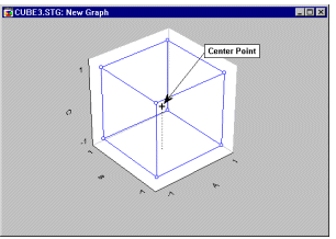
Later in the analysis (see below), one can compare the measurements for the dependent variable at the center point with the average for the rest of the design. This provides a check for curvature (see Box and Draper, 1987): If the mean for the dependent variable at the center of the design is significantly different from the overall mean at all other points of the design, then one has good reason to believe that the simple assumption that the factors are linearly related to the dependent variable, does not hold.
Analyzing the Results of a 2**(k-p) Experiment
Analysis of variance. Next, one needs to determine exactly which of the factors significantly affected the dependent variable of interest. For example, in the study reported by Box and Draper (1987, page 115), it is desired to learn which of the factors involved in the manufacture of dyestuffs affected the strength of the fabric. In this example, factors 1 (Polysulfide), 4 (Time), and 6 (Temperature) significantly affected the strength of the fabric. Note that to simplify matters, only main effects are shown below.
| ANOVA; Var.:STRENGTH; R-sqr = .60614; Adj:.56469 (fabrico.sta) | |||||
|---|---|---|---|---|---|
| 2**(6-0) design; MS Residual = 3.62509 DV: STRENGTH |
|||||
| SS | df | MS | F | p | |
| (1)POLYSUFD (2)REFLUX (3)MOLES (4)TIME (5)SOLVENT (6)TEMPERTR Error Total SS |
48.8252 7.9102 .1702 142.5039 2.7639 115.8314 206.6302 524.6348 |
1 1 1 1 1 1 57 63 |
48.8252 7.9102 .1702 142.5039 2.7639 115.8314 3.6251 |
13.46867 2.18206 .04694 39.31044 .76244 31.95269 |
.000536 .145132 .829252 .000000 .386230 .000001 |
Pure error and lack of fit. If the experimental design is at least partially replicated, then one can estimate the error variability for the experiment from the variability of the replicated runs. Since those measurements were taken under identical conditions, that is, at identical settings of the factor levels, the estimate of the error variability from those runs is independent of whether or not the "true" model is linear or non-linear in nature, or includes higher-order interactions. The error variability so estimated represents pure error, that is, it is entirely due to unreliabilities in the measurement of the dependent variable. If available, one can use the estimate of pure error to test the significance of the residual variance, that is, all remaining variability that cannot be accounted for by the factors and their interactions that are currently in the model. If, in fact, the residual variability is significantly larger than the pure error variability, then one can conclude that there is still some statistically significant variability left that is attributable to differences between the groups, and hence, that there is an overall lack of fit of the current model.
| ANOVA; Var.:STRENGTH; R-sqr = .58547; Adj:.56475 (fabrico.sta) | |||||
|---|---|---|---|---|---|
| 2**(3-0) design; MS Pure Error = 3.594844 DV: STRENGTH |
|||||
| SS | df | MS | F | p | |
| (1)POLYSUFD (2)TIME (3)TEMPERTR Lack of Fit Pure Error Total SS |
48.8252 142.5039 115.8314 16.1631 201.3113 524.6348 |
1 1 1 4 56 63 |
48.8252 142.5039 115.8314 4.0408 3.5948 |
13.58200 39.64120 32.22154 1.12405 |
.000517 .000000 .000001 .354464 |
For example, the table above shows the results for the three factors that were previously identified as most important in their effect on fabric strength; all other factors where ignored in the analysis. As you can see in the row with the label Lack of Fit, when the residual variability for this model (i.e., after removing the three main effects) is compared against the pure error estimated from the within-group variability, the resulting F test is not statistically significant. Therefore, this result additionally supports the conclusion that, indeed, factors Polysulfide, Time, and Temperature significantly affected resultant fabric strength in an additive manner (i.e., there are no interactions). Or, put another way, all differences between the means obtained in the different experimental conditions can be sufficiently explained by the simple additive model for those three variables.
Parameter or effect estimates. Now, look at how these factors affected the strength of the fabrics.
| Effect | Std.Err. | t (57) | p | |
|---|---|---|---|---|
| Mean/Interc. (1)POLYSUFD (2)REFLUX (3)MOLES (4)TIME (5)SOLVENT (6)TEMPERTR |
11.12344 1.74688 .70313 .10313 2.98438 -.41562 2.69062 |
.237996 .475992 .475992 .475992 .475992 .475992 .475992 |
46.73794 3.66997 1.47718 .21665 6.26980 -.87318 5.65267 |
.000000 .000536 .145132 .829252 .000000 .386230 .000001 |
The numbers above are the effect or parameter estimates. With the exception of the overall Mean/Intercept, these estimates are the deviations of the mean of the negative settings from the mean of the positive settings for the respective factor. For example, if you change the setting of factor Time from low to high, then you can expect an improvement in Strength by 2.98; if you set the value for factor Polysulfd to its high setting, you can expect a further improvement by 1.75, and so on.
As you can see, the same three factors that were statistically significant show the largest parameter estimates; thus the settings of these three factors were most important for the resultant strength of the fabric.
For analyses including interactions, the interpretation of the effect parameters is a bit more complicated. Specifically, the two-way interaction parameters are defined as half the difference between the main effects of one factor at the two levels of a second factor (see Mason, Gunst, and Hess, 1989, page 127); likewise, the three-way interaction parameters are defined as half the difference between the two-factor interaction effects at the two levels of a third factor, and so on.
Regression coefficients. One can also look at the parameters in the multiple regression model (see Multiple Regression). To continue this example, consider the following prediction equation:
Strength = const + b1 *x1 +... + b6 *x6
Here x1 through x6 stand for the 6 factors in the analysis. The Effect Estimates shown earlier also contains these parameter estimates:
| Coeff. |
Std.Err. Coeff. |
-95.% Cnf.Limt |
+95.% Cnf.Limt |
|
|---|---|---|---|---|
| Mean/Interc. (1)POLYSUFD (2)REFLUX (3)MOLES (4)TIME (5)SOLVENT (6)TEMPERTR |
11.12344 .87344 .35156 .05156 1.49219 -.20781 1.34531 |
.237996 .237996 .237996 .237996 .237996 .237996 .237996 |
10.64686 .39686 -.12502 -.42502 1.01561 -.68439 .86873 |
11.60002 1.35002 .82814 .52814 1.96877 .26877 1.82189 |
Actually, these parameters contain little "new" information, as they simply are one-half of the parameter values (except for the Mean/Intercept) shown earlier. This makes sense since now, the coefficient can be interpreted as the deviation of the high-setting for the respective factors from the center. However, note that this is only the case if the factor values (i.e., their levels) are coded as -1 and +1, respectively. Otherwise, the scaling of the factor values will affect the magnitude of the parameter estimates. In the example data reported by Box and Draper (1987, page 115), the settings or values for the different factors were recorded on very different scales:
| data file: FABRICO.STA [ 64 cases with 9 variables ] 2**(6-0) Design, Box & Draper, p. 117 |
|||||||||
|---|---|---|---|---|---|---|---|---|---|
| POLYSUFD | REFLUX | MOLES | TIME | SOLVENT | TEMPERTR | STRENGTH | HUE | BRIGTHNS | |
| 1 2 3 4 5 6 7 8 9 10 11 12 13 14 15 . . . |
6 7 6 7 6 7 6 7 6 7 6 7 6 7 6 . . . |
150 150 170 170 150 150 170 170 150 150 170 170 150 150 170 . . . |
1.8 1.8 1.8 1.8 2.4 2.4 2.4 2.4 1.8 1.8 1.8 1.8 2.4 2.4 2.4 . . . |
24 24 24 24 24 24 24 24 36 36 36 36 36 36 36 . . . |
30 30 30 30 30 30 30 30 30 30 30 30 30 30 30 . . . |
120 120 120 120 120 120 120 120 120 120 120 120 120 120 120 . . . |
3.4 9.7 7.4 10.6 6.5 7.9 10.3 9.5 14.3 10.5 7.8 17.2 9.4 12.1 9.5 . . . |
15.0 5.0 23.0 8.0 20.0 9.0 13.0 5.0 23.0 1.0 11.0 5.0 15.0 8.0 15.0 . . . |
36.0 35.0 37.0 34.0 30.0 32.0 28.0 38.0 40.0 32.0 32.0 28.0 34.0 26.0 30.0 . . . |
Shown below are the regression coefficient estimates based on the uncoded original factor values:
| Regressn Coeff. |
Std.Err. |
t (57) |
p |
|
|---|---|---|---|---|
| Mean/Interc. (1)POLYSUFD (2)REFLUX (3)MOLES (4)TIME (5)SOLVENT (6)TEMPERTR |
-46.0641 1.7469 .0352 .1719 .2487 -.0346 .2691 |
8.109341 .475992 .023800 .793320 .039666 .039666 .047599 |
-5.68037 3.66997 1.47718 .21665 6.26980 -.87318 5.65267 |
.000000 .000536 .145132 .829252 .000000 .386230 .000001 |
Because the metric for the different factors is no longer compatible, the magnitudes of the regression coefficients are not compatible either. This is why it is usually more informative to look at the ANOVA parameter estimates (for the coded values of the factor levels), as shown before. However, the regression coefficients can be useful when one wants to make predictions for the dependent variable, based on the original metric of the factors.
Graph Options
Diagnostic plots of residuals. To start with, before accepting a particular "model" that includes a particular number of effects (e.g., main effects for Polysulfide, Time, and Temperature in the current example), one should always examine the distribution of the residual values. These are computed as the difference between the predicted values (as predicted by the current model) and the observed values. You can compute the histogram for these residual values, as well as probability plots (as shown below).
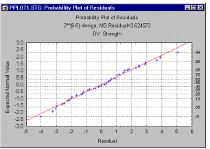
The parameter estimates and ANOVA table are based on the assumption that the residuals are normally distributed (see also Elementary Concepts). The histogram provides one way to check (visually) whether this assumption holds. The so-called normal probability plot is another common tool to assess how closely a set of observed values (residuals in this case) follows a theoretical distribution. In this plot the actual residual values are plotted along the horizontal X-axis; the vertical Y-axis shows the expected normal values for the respective values, after they were rank-ordered. If all values fall onto a straight line, then one can be satisfied that the residuals follow the normal distribution.
Pareto chart of effects. The Pareto chart of effects is often an effective tool for communicating the results of an experiment, in particular to laymen.
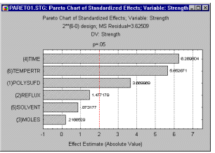
In this graph, the ANOVA effect estimates are sorted from the largest absolute value to the smallest absolute value. The magnitude of each effect is represented by a column, and often, a line going across the columns indicates how large an effect has to be (i.e., how long a column must be) to be statistically significant.
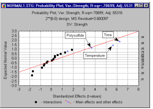
Normal probability plot of effects. Another useful, albeit more technical summary graph, is the normal probability plot of the estimates. As in the normal probability plot of the residuals, first the effect estimates are rank ordered, and then a normal z score is computed based on the assumption that the estimates are normally distributed. This z score is plotted on the Y-axis; the observed estimates are plotted on the X-axis (as shown below).
Square and cube plots. These plots are often used to summarize predicted values for the dependent variable, given the respective high and low setting of the factors. The square plot (see below) will show the predicted values (and, optionally, their confidence intervals) for two factors at a time. The cube plot will show the predicted values (and, optionally, confidence intervals) for three factors at a time.
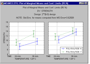
Interaction plots. A general graph for showing the means is the standard interaction plot, where the means are indicated by points connected by lines. This plot (see below) is particularly useful when there are significant interaction effects in the model.
Surface and contour plots. When the factors in the design are continuous in nature, it is often also useful to look at surface and contour plots of the dependent variable as a function of the factors.
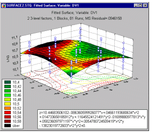
These types of plots will further be discussed later in this section, in the context of 3**(k-p), and central composite and response surface designs.
Summary
2**(k-p) designs are the "workhorse" of industrial experiments. The impact of a large number of factors on the production process can simultaneously be assessed with relative efficiency (i.e., with few experimental runs). The logic of these types of experiments is straightforward (each factor has only two settings).
Disadvantages. The simplicity of these designs is also their major flaw. As mentioned before, underlying the use of two-level factors is the belief that the resultant changes in the dependent variable (e.g., fabric strength) are basically linear in nature. This is often not the case, and many variables are related to quality characteristics in a non-linear fashion. In the example above, if you were to continuously increase the temperature factor (which was significantly related to fabric strength), you would of course eventually hit a "peak," and from there on the fabric strength would decrease as the temperature increases. While this types of curvature in the relationship between the factors in the design and the dependent variable can be detected if the design included center point runs, one cannot fit explicit nonlinear (e.g., quadratic) models with 2**(k-p) designs (however, central composite designs will do exactly that).
Another problem of fractional designs is the implicit assumption that higher-order interactions do not matter; but sometimes they do, for example, when some other factors are set to a particular level, temperature may be negatively related to fabric strength. Again, in fractional factorial designs, higher-order interactions (greater than two-way) particularly will escape detection.
| To index |
2**(k-p) fractional factorial designs are often used in industrial experimentation because of the economy of data collection that they provide. For example, suppose an engineer needed to investigate the effects of varying 11 factors, each with 2 levels, on a manufacturing process. Let us call the number of factors k, which would be 11 for this example. An experiment using a full factorial design, where the effects of every combination of levels of each factor are studied, would require 2**(k) experimental runs, or 2048 runs for this example. To minimize the data collection effort, the engineer might decide to forego investigation of higher-order interaction effects of the 11 factors, and focus instead on identifying the main effects of the 11 factors and any low-order interaction effects that could be estimated from an experiment using a smaller, more reasonable number of experimental runs. There is another, more theoretical reason for not conducting huge, full factorial 2 level experiments. In general, it is not logical to be concerned with identifying higher-order interaction effects of the experimental factors, while ignoring lower-order nonlinear effects, such as quadratic or cubic effects, which cannot be estimated if only 2 levels of each factor are employed. So althrough practical considerations often lead to the need to design experiments with a reasonably small number of experimental runs, there is a logical justification for such experiments.
The alternative to the 2**(k) full factorial design is the 2**(k-p) fractional factorial design, which requires only a "fraction" of the data collection effort required for full factorial designs. For our example with k=11 factors, if only 64 experimental runs can be conducted, a 2**(11-5) fractional factorial experiment would be designed with 2**6 = 64 experimental runs. In essence, a k-p = 6 way full factorial experiment is designed, with the levels of the p factors being "generated" by the levels of selected higher order interactions of the other 6 factors. Fractional factorials "sacrifice" higher order interaction effects so that lower order effects may still be computed correctly. However, different criteria can be used in choosing the higher order interactions to be used as generators, with different criteria sometimes leading to different "best" designs.
2**(k-p) fractional factorial designs can also include blocking factors. In some production processes, units are produced in natural "chunks" or blocks. To make sure that these blocks do not bias your estimates of the effects for the k factors, blocking factors can be added as additional factors in the design. Consequently, you may "sacrifice" additional interaction effects to generate the blocking factors, but these designs often have the advantage of being statistically more powerful, because they allow you to estimate and control the variability in the production process that is due to differences between blocks.
Design Criteria
Many of the concepts discussed in this overview are also addressed in the Overview of 2**(k-p) Fractional factorial designs. However, a technical description of how fractional factorial designs are constructed is beyond the scope of either introductory overview. Detailed accounts of how to design 2**(k-p) experiments can be found, for example, in Bayne and Rubin (1986), Box and Draper (1987), Box, Hunter, and Hunter (1978), Montgomery (1991), Daniel (1976), Deming and Morgan (1993), Mason, Gunst, and Hess (1989), or Ryan (1989), to name only a few of the many text books on this subject.
In general, the 2**(k-p) maximally unconfounded and minimum aberration designs techniques will successively select which higher-order interactions to use as generators for the p factors. For example, consider the following design that includes 11 factors but requires only 16 runs (observations).
| Design: 2**(11-7), Resolution III | |||||||||||
|---|---|---|---|---|---|---|---|---|---|---|---|
| Run | A | B | C | D | E | F | G | H | I | J | K |
| 1 2 3 4 5 6 7 8 9 10 11 12 13 14 15 16 |
1 1 1 1 1 1 1 1 -1 -1 -1 -1 -1 -1 -1 -1 |
1 1 1 1 -1 -1 -1 -1 1 1 1 1 -1 -1 -1 -1 |
1 1 -1 -1 1 1 -1 -1 1 1 -1 -1 1 1 -1 -1 |
1 -1 1 -1 1 -1 1 -1 1 -1 1 -1 1 -1 1 -1 |
1 1 -1 -1 -1 -1 1 1 -1 -1 1 1 1 1 -1 -1 |
1 -1 -1 1 -1 1 1 -1 1 -1 -1 1 -1 1 1 -1 |
1 -1 -1 1 1 -1 -1 1 -1 1 1 -1 -1 1 1 -1 |
1 -1 1 -1 -1 1 -1 1 -1 1 -1 1 1 -1 1 -1 |
1 -1 -1 1 -1 1 1 -1 -1 1 1 -1 1 -1 -1 1 |
1 1 1 1 -1 -1 -1 -1 -1 -1 -1 -1 1 1 1 1 |
1 1 -1 -1 1 1 -1 -1 -1 -1 1 1 -1 -1 1 1 |
Interpreting the design. The design displayed in the Scrollsheet above should be interpreted as follows. Each column contains +1's or -1's to indicate the setting of the respective factor (high or low, respectively). So for example, in the first run of the experiment, all factors A through K are set to the higher level, and in the second run, factors A, B, and C are set to the higher level, but factor D is set to the lower level, and so on. Notice that the settings for each experimental run for factor E can be produced by multiplying the respective settings for factors A, B, and C. The A x B x C interaction effect therefore cannot be estimated independently of the factor E effect in this design because these two effects are confounded. Likewise, the settings for factor F can be produced by multiplying the respective settings for factors B, C, and D. We say that ABC and BCD are the generators for factors E and F, respectively.
The maximum resolution design criterion. In the Scrollsheet shown above, the design is described as a 2**(11-7) design of resolution III (three). This means that you study overall k = 11 factors, but p = 7 of those factors were generated from the interactions of a full 2**[(11-7) = 4] factorial design. As a result, the design does not give full resolution; that is, there are certain interaction effects that are confounded with (identical to) other effects. In general, a design of resolution R is one where no l-way interactions are confounded with any other interaction of order less than R - l. In the current example, R is equal to 3. Here, no l = 1-way interactions (i.e., main effects) are confounded with any other interaction of order less than R - l = 3 -1 = 2. Thus, main effects in this design are unconfounded with each other, but are confounded with two-factor interactions; and consequently, with other higher-order interactions. One obvious, but nevertheless very important overall design criterion is that the higher-order interactions to be used as generators should be chosen such that the resolution of the design is as high as possible.
The maximum unconfounding design criterion. Maximizing the resolution of a design, however, does not by itself ensure that the selected generators produce the "best" design. Consider, for example, two different resolution IV designs. In both designs, main effects would be unconfounded with each other and 2-factor interactions would be unconfounded with main effects, i.e, no l = 2-way interactions are confounded with any other interaction of order less than R - l = 4 - 2 = 2. The two designs might be different, however, with regard to the degree of confounding for the 2-factor interactions. For resolution IV designs, the "crucial order," in which confounding of effects first appears, is for 2-factor interactions. In one design, none of the "crucial order," 2-factor interactions might be unconfounded with all other 2-factor interactions, while in the other design, virtually all of the 2-factor interactions might be unconfounded with all of the other 2-factor interactions. The second "almost resolution V" design would be preferable to the first "just barely resolution IV" design. This suggests that even though the maximum resolution design criterion should be the primary criterion, a subsidiary criterion might be that generators should be chosen such that the maximum number of interactions of less than or equal to the crucial order, given the resolution, are unconfounded with all other interactions of the crucial order. This is called the maximum unconfounding design criterion, and is one of the optional, subsidiary design criterion to use in a search for a 2**(k-p) design.
The minimum aberration design criterion. The miniminum aberration design criterion is another optional, subsidiary criterion to use in a search for a 2**(k-p) design. In some respects, this criterion is similar to the maximum unconfounding design criterion. Technically, the minimum aberration design is defined as the design of maximum resolution "which minimizes the number of words in the defining relation that are of minimum length" (Fries & Hunter, 1980). Less technically, the criterion apparently operates by choosing generators that produce the smallest number of pairs of confounded interactions of the crucial order. For example, the minimum aberration resolution IV design would have the minimum number of pairs of confounded 2-factor interactions.
To illustrate the difference between the maximum unconfounding and minimum aberration criteria, consider the maximally unconfounded 2**(9-4) design and the minimum aberration 2**(9-4) design, as for example, listed in Box, Hunter, and Hunter (1978). If you compare these two designs, you will find that in the maximally unconfounded design, 15 of the 36 2-factor interactions are unconfounded with any other 2-factor interactions, while in the minimum aberration design, only 8 of the 36 2-factor interactions are unconfounded with any other 2-factor interactions. The minimum aberration design, however, produces 18 pairs of confounded interactions, while the maximally unconfounded design produces 21 pairs of confounded interactions. So, the two criteria lead to the selection of generators producing different "best" designs.
Fortunately, the choice of whether to use the maximum unconfounding criterion or the minimum aberration criterion makes no difference in the design which is selected (except for, perhaps, relabeling of the factors) when there are 11 or fewer factors, with the single exception of the 2**(9-4) design described above (see Chen, Sun, & Wu, 1993). For designs with more than 11 factors, the two criteria can lead to the selection of very different designs, and for lack of better advice, we suggest using both criteria, comparing the designs that are produced, and choosing the design that best suits your needs. We will add, editorially, that maximizing the number of totally unconfounded effects often makes more sense than minimizing the number of pairs of confounded effects.
Summary
2**(k-p) fractional factorial designs are probably the most frequently used type of design in industrial experimentation. Things to consider in designing any 2**(k-p) fractional factorial experiment include the number of factors to be investigated, the number of experimental runs, and whether there will be blocks of experimental runs. Beyond these basic considerations, one should also take into account whether the number of runs will allow a design of the required resolution and degree of confounding for the crucial order of interactions, given the resolution.
| To index |
In some cases, factors that have more than 2 levels have to be examined. For example, if one suspects that the effect of the factors on the dependent variable of interest is not simply linear, then, as discussed earlier (see 2**(k-p) designs), one needs at least 3 levels in order to test for the linear and quadratic effects (and interactions) for those factors. Also, sometimes some factors may be categorical in nature, with more than 2 categories. For example, you may have three different machines that produce a particular part.
Designing 3**(k-p) Experiments
The general mechanism of generating fractional factorial designs at 3 levels (3**(k-p) designs) is very similar to that described in the context of 2**(k-p) designs. Specifically, one starts with a full factorial design, and then uses the interactions of the full design to construct "new" factors (or blocks) by making their factor levels identical to those for the respective interaction terms (i.e., by making the new factors aliases of the respective interactions).
For example, consider the following simple 3**(3-1) factorial design:
| 3**(3-1) fractional factorial design, 1 block , 9 runs |
|||
|---|---|---|---|
| Standard Run |
A |
B |
C |
| 1 2 3 4 5 6 7 8 9 |
0 0 0 1 1 1 2 2 2 |
0 1 2 0 1 2 0 1 2 |
0 2 1 2 1 0 1 0 2 |
As in the case of 2**(k-p) designs, the design is constructed by starting with the full 3-1=2 factorial design; those factors are listed in the first two columns (factors A and B). Factor C is constructed from the interaction AB of the first two factors. Specifically, the values for factor C are computed as
C = 3 - mod3 (A+B)
Here, mod3(x) stands for the so-called modulo-3 operator, which will first find a number y that is less than or equal to x, and that is evenly divisible by 3, and then compute the difference (remainder) between number y and x. For example, mod3(0) is equal to 0, mod3(1) is equal to 1, mod3(3) is equal to 0, mod3(5) is equal to 2 (3 is the largest number that is less than or equal to 5, and that is evenly divisible by 3; finally, 5-3=2), and so on.
Fundamental identity. If you apply this function to the sum of columns A and B shown above, you will obtain the third column C. Similar to the case of 2**(k-p) designs (see 2**(k-p) designs for a discussion of the fundamental identity in the context of 2**(k-p) designs), this confounding of interactions with "new" main effects can be summarized in an expression:
0 = mod3 (A+B+C)
If you look back at the 3**(3-1) design shown earlier, you will see that, indeed, if you add the numbers in the three columns they will all sum to either 0, 3, or 6, that is, values that are evenly divisible by 3 (and hence: mod3(A+B+C)=0). Thus, one could write as a shortcut notation ABC=0, in order to summarize the confounding of factors in the fractional 3**(k-p) design.
Some of the designs will have fundamental identities that contain the number 2 as a multiplier; e.g.,
0 = mod3 (B+C*2+D+E*2+F)
This notation can be interpreted exactly as before, that is, the modulo3 of the sum B+2*C+D+2*E+F must be equal to 0. The next example shows such an identity.
An Example 3**(4-1) Design in 9 Blocks
Here is the summary for a 4-factor 3-level fractional factorial design in 9 blocks, that requires only 27 runs.
SUMMARY: 3**(4-1) fractional factorial
Design generators: ABCD
Block generators: AB,AC2
Number of factors (independent variables): 4
Number of runs (cases, experiments): 27
Number of blocks: 9
This design will allow you to test for linear and quadratic main effects for 4 factors in 27 observations, which can be gathered in 9 blocks of 3 observations each. The fundamental identity or design generator for the design is ABCD, thus the modulo3 of the sum of the factor levels across the four factors is equal to 0. The fundamental identity also allows you to determine the confounding of factors and interactions in the design (see McLean and Anderson, 1984, for details).
| Unconfounded Effects (experi3.sta) | ||
|---|---|---|
| EXPERIM. DESIGN |
List of uncorrelated factors and interactions 3**(4-1) fractional factorial design, 9 blocks, 27 runs |
|
| Unconf. Effects (excl. blocks) |
Unconfounded if blocks included? |
|
| 1 2 3 4 5 6 7 8 |
(1)A (L) A (Q) (2)B (L) B (Q) (3)C (L) C (Q) (4)D (L) D (Q) |
Yes Yes Yes Yes Yes Yes Yes Yes |
As you can see, in this 3**(4-1) design the main effects are not confounded with each other, even when the experiment is run in 9 blocks.
Box-Behnken Designs
In the case of 2**(k-p) designs, Plackett and Burman (1946) developed highly fractionalized designs to screen the maximum number of (main) effects in the least number of experimental runs. The equivalent in the case of 3**(k-p) designs are the so-called Box-Behnken designs (Box and Behnken, 1960; see also Box and Draper, 1984). These designs do not have simple design generators (they are constructed by combining two-level factorial designs with incomplete block designs), and have complex confounding of interaction. However, the designs are economical and therefore particularly useful when it is expensive to perform the necessary experimental runs.
Analyzing the 3**(k-p) Design
The analysis of these types of designs proceeds basically in the same way as was described in the context of 2**(k-p) designs. However, for each effect, one can now test for the linear effect and the quadratic (non-linear effect). For example, when studying the yield of chemical process, then temperature may be related in a non-linear fashion, that is, the maximum yield may be attained when the temperature is set at the medium level. Thus, non-linearity often occurs when a process performs near its optimum.
ANOVA Parameter Estimates
To estimate the ANOVA parameters, the factors levels for the factors in the analysis are internally recoded so that one can test the linear and quadratic components in the relationship between the factors and the dependent variable. Thus, regardless of the original metric of factor settings (e.g., 100 degrees C, 110 degrees C, 120 degrees C), you can always recode those values to -1, 0, and +1 to perform the computations. The resultant ANOVA parameter estimates can be interpreted analogously to the parameter estimates for 2**(k-p) designs.
For example, consider the following ANOVA results:
| Factor | Effect | Std.Err. | t (69) | p |
|---|---|---|---|---|
| Mean/Interc. BLOCKS(1) BLOCKS(2) (1)TEMPERAT (L) TEMPERAT (Q) (2)TIME (L) TIME (Q) (3)SPEED (L) SPEED (Q) 1L by 2L 1L by 2Q 1Q by 2L 1Q by 2Q |
103.6942 .8028 -1.2307 -.3245 -.5111 .0017 .0045 -10.3073 -3.7915 3.9256 .4384 .4747 -2.7499 |
.390591 1.360542 1.291511 .977778 .809946 .977778 .809946 .977778 .809946 1.540235 1.371941 1.371941 .995575 |
265.4805 .5901 -.9529 -.3319 -.6311 .0018 .0056 -10.5415 -4.6812 2.5487 .3195 .3460 -2.7621 |
0.000000 .557055 .343952 .740991 .530091 .998589 .995541 .000000 .000014 .013041 .750297 .730403 .007353 |
Main-effect estimates. By default, the Effect estimate for the linear effects (marked by the L next to the factor name) can be interpreted as the difference between the average response at the low and high settings for the respective factors. The estimate for the quadratic (non-linear) effect (marked by the Q next to the factor name) can be interpreted as the difference between the average response at the center (medium) settings and the combined high and low settings for the respective factors.
Interaction effect estimates. As in the case of 2**(k-p) designs, the linear-by-linear interaction effect can be interpreted as half the difference between the linear main effect of one factor at the high and low settings of another. Analogously, the interactions by the quadratic components can be interpreted as half the difference between the quadratic main effect of one factor at the respective settings of another; that is, either the high or low setting (quadratic by linear interaction), or the medium or high and low settings combined (quadratic by quadratic interaction).
In practice, and from the standpoint of "interpretability of results," one would usually try to avoid quadratic interactions. For example, a quadratic-by-quadratic A-by-B interaction indicates that the non- linear effect of factor A is modified in a nonlinear fashion by the setting of B. This means that there is a fairly complex interaction between factors present in the data, that will make it difficult to understand and optimize the respective process. Sometimes, performing nonlinear transformations (e.g., performing a log transformation) of the dependent variable values can remedy the problem.
Centered and non-centered polynomials. As mentioned above, the interpretation of the effect estimates applies only when you use the default parameterization of the model. In that case, the you will code the quadratic factor interactions, so that they become maximally "untangled" from the linear main effects.
Graphical Presentation of Results
The same diagnostic plots (e.g., of residuals) are available for 3**(k-p) designs as were described in the context of 2**(k-p) designs. Thus, before interpreting the final results, one should always first look at the distribution of the residuals for the final fitted model. The ANOVA assumes that the residuals (errors) are normally distributed.
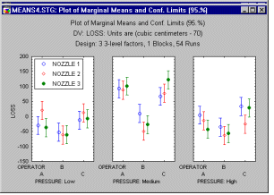
Plot of means. When an interaction involves categorical factors (e.g., type of machine, specific operator of machine, and some distinct setting of the machine), then the best way to understand interactions is to look at the respective interaction plot of means.
Surface plot. When the factors in an interaction are continuous in nature, you may want to look at the surface plot that shows the response surface applied by the fitted model. Note that this graph also contains the prediction equation (in terms of the original metric of factors), that produces the respective response surface.
Designs for Factors at 2 and 3 Levels
You can also generate standard designs with 2 and 3 level factors. Specifically, you can generate the standard designs as enumerated by Connor and Young for the US National Bureau of Standards (see McLean and Anderson, 1984). The technical details of the method used to generate these designs are beyond the scope of this introduction. However, in general the technique is, in a sense, a combination of the procedures described in the context of 2**(k-p) and 3**(k-p) designs. It should be noted however, that, while all of these designs are very efficient, they are not necessarily orthogonal with respect to all main effects. This is, however, not a problem, if one uses a general algorithm for estimating the ANOVA parameters and sums of squares, that does not require orthogonality of the design.
The design and analysis of these experiments proceeds along the same lines as discussed in the context of 2**(k-p) and 3**(k-p) experiments.
| To index |
The 2**(k-p) and 3**(k-p) designs all require that the levels of the factors are set at, for example, 2 or 3 levels. In many instances, such designs are not feasible, because, for example, some factor combinations are constrained in some way (e.g., factors A and B cannot be set at their high levels simultaneously). Also, for reasons related to efficiency, which will be discussed shortly, it is often desirable to explore the experimental region of interest at particular points that cannot be represented by a factorial design.
The designs (and how to analyze them) discussed in this section all pertain to the estimation (fitting) of response surfaces, following the general model equation:
y = b0 +b1 *x1 +...+bk *xk + b12 *x1 *x2 +b13 *x1 *x3 +...+bk-1,k *xk-1 *xk + b11 *x1² +...+bkk *xk²
Put into words, one is fitting a model to the observed values of the dependent variable y, that include (1) main effects for factors x1 , ..., xk, (2) their interactions (x1*x2, x1*x3, ... ,xk-1*xk), and (3) their quadratic components (x1**2, ..., xk**2). No assumptions are made concerning the "levels" of the factors, and you can analyze any set of continuous values for the factors.
There are some considerations concerning design efficiency and biases, which have led to standard designs that are ordinarily used when attempting to fit these response surfaces, and those standard designs will be discussed shortly (e.g., see Box, Hunter, and Hunter, 1978; Box and Draper, 1987; Khuri and Cornell, 1987; Mason, Gunst, and Hess, 1989; Montgomery, 1991). But, as will be discussed later, in the context of constrained surface designs and D- and A-optimal designs, these standard designs can sometimes not be used for practical reasons. However, the central composite design analysis options do not make any assumptions about the structure of your data file, that is, the number of distinct factor values, or their combinations across the runs of the experiment, and, hence, these options can be used to analyze any type of design, to fit to the data the general model described above.
Design Considerations
Orthogonal designs. One desirable characteristic of any design is that the main effect and interaction estimates of interest are independent of each other. For example, suppose you had a two- factor experiments, with both factors at two levels. Your design consists of four runs:
| A | B | |
|---|---|---|
| Run 1 Run 2 Run 3 Run 4 |
1 1 -1 -1 |
1 1 -1 -1 |
For the first two runs, both factors A and B are set at their high levels (+1). In the last two runs, both are set at their low levels (-1). Suppose you wanted to estimate the independent contributions of factors A and B to the prediction of the dependent variable of interest. Clearly this is a silly design, because there is no way to estimate the A main effect and the B main effect. One can only estimate one effect -- the difference between Runs 1+2 vs. Runs 3+4 -- which represents the combined effect of A and B.
The point here is that, in order to assess the independent contributions of the two factors, the factor levels in the four runs must be set so that the "columns" in the design (under A and B in the illustration above) are independent of each other. Another way to express this requirement is to say that the columns of the design matrix (with as many columns as there are main effect and interaction parameters that one wants to estimate) should be orthogonal (this term was first used by Yates, 1933). For example, if the four runs in the design are arranged as follows:
| A | B | |
|---|---|---|
| Run 1 Run 2 Run 3 Run 4 |
1 1 -1 -1 |
1 -1 1 -1 |
then the A and B columns are orthogonal. Now you can estimate the A main effect by comparing the high level for A within each level of B, with the low level for A within each level of B; the B main effect can be estimated in the same way.
Technically, two columns in a design matrix are orthogonal if the sum of the products of their elements within each row is equal to zero. In practice, one often encounters situations, for example due to loss of some data in some runs or other constraints, where the columns of the design matrix are not completely orthogonal. In general, the rule here is that the more orthogonal the columns are, the better the design, that is, the more independent information can be extracted from the design regarding the respective effects of interest. Therefore, one consideration for choosing standard central composite designs is to find designs that are orthogonal or near-orthogonal.
Rotatable designs. The second consideration is related to the first requirement, in that it also has to do with how best to extract the maximum amount of (unbiased) information from the design, or specifically, from the experimental region of interest. Without going into details (see Box, Hunter, and Hunter, 1978; Box and Draper, 1987, Chapters 14; see also Deming and Morgan, 1993, Chapter 13), it can be shown that the standard error for the prediction of dependent variable values is proportional to:
(1 + f(x)' * (X'X)¨¹ * f(x))**½
where f(x) stands for the (coded) factor effects for the respective model (f(x) is a vector, f(x)' is the transpose of that vector), and X is the design matrix for the experiment, that is, the matrix of coded factor effects for all runs; X'X**-1 is the inverse of the crossproduct matrix. Deming and Morgan (1993) refer to this expression as the normalized uncertainty; this function is also related to the variance function as defined by Box and Draper (1987). The amount of uncertainty in the prediction of dependent variable values depends on the variability of the design points, and their covariance over the runs. (Note that it is inversely proportional to the determinant of X'X; this issue is further discussed in the section on D- and A-optimal designs).
The point here is that, again, one would like to choose a design that extracts the most information regarding the dependent variable, and leaves the least amount of uncertainty for the prediction of future values. It follows, that the amount of information (or normalized information according to Deming and Morgan, 1993) is the inverse of the normalized uncertainty.
For the simple 4-run orthogonal experiment shown earlier, the information function is equal to
Ix = 4/(1 + x1² + x2²)
where x1 and x2 stand for the factor settings for factors A and B, respectively (see Box and Draper, 1987).
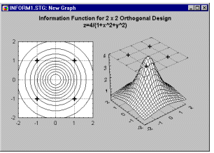
Inspection of this function in a plot (see above) shows that it is constant on circles centered at the origin. Thus any kind of rotation of the original design points will generate the same amount of information, that is, generate the same information function. Therefore, the 2-by-2 orthogonal design in 4 runs shown earlier is said to be rotatable.
As pointed out before, in order to estimate the second order, quadratic, or non-linear component of the relationship between a factor and the dependent variable, one needs at least 3 levels for the respective factors. What does the information function look like for a simple 3-by-3 factorial design, for the second-order quadratic model as shown at the beginning of this section?
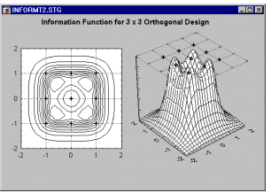
As it turns out (see Box and Draper, 1987 and Montgomery, 1991; refer also to the manual), this function looks more complex, contains "pockets" of high-density information at the edges (which are probably of little particular interest to the experimenter), and clearly it is not constant on circles around the origin. Therefore, it is not rotatable, meaning different rotations of the design points will extract different amounts of information from the experimental region.
Star-points and rotatable second-order designs. It can be shown that by adding so-called star- points to the simple (square or cube) 2-level factorial design points, one can achieve rotatable, and often orthogonal or nearly orthogonal designs. For example, adding to the simple 2-by-2 orthogonal design shown earlier the following points, will produce a rotatable design.
| A | B | |
|---|---|---|
| Run 1 Run 2 Run 3 Run 4 Run 5 Run 6 Run 7 Run 8 Run 9 Run 10 |
1 1 -1 -1 -1.414 1.414 0 0 0 0 |
1 -1 1 -1 0 0 -1.414 1.414 0 0 |
The first four runs in this design are the previous 2-by-2 factorial design points (or square points or cube points); runs 5 through 8 are the so-called star points or axial points, and runs 9 and 10 are center points.
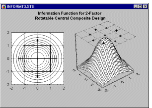
The information function for this design for the second-order (quadratic) model is rotatable, that is, it is constant on the circles around the origin.
Alpha for Rotatability and Orthogonality
The two design characteristics discussed so far -- orthogonality and rotatability -- depend on the number of center points in the design and on the so-called axial distance (alpha), which is the distance of the star points from the center of the design (i.e., 1.414 in the design shown above). It can be shown (e.g., see Box, Hunter, and Hunter, 1978; Box and Draper, 1987, Khuri and Cornell, 1987; Montgomery, 1991) that a design is rotatable if:
 = ( nc )¼
where nc stands for the number of cube points in the design (i.e., points in the factorial portion of the design).
A central composite design is orthogonal, if one chooses the axial distance so that:
 = {[( nc + ns + n0 )½ - nc½]² * nc/4}¼
where
nc is the number of cube points in the design
ns is the number of star points in the design
n0 is the number of center points in the design
To make a design both (approximately) orthogonal and rotatable, one would first choose the axial distance for rotatability, and then add center points (see Kkuri and Cornell, 1987), so that:
n0  4*nc½ + 4 - 2k
where k stands for the number of factors in the design.
Finally, if blocking is involved, Box and Draper (1987) give the following formula for computing the axial distance to achieve orthogonal blocking, and in most cases also reasonable information function contours, that is, contours that are close to spherical:
 = [k*(l+ns0/ns)/(1+nc0/nc)]½
where
ns0 is the number of center points in the star portion of the design
ns is the number of non-center star points in the design
nc0 is the number of center points in the cube portion of the design
nc is the number of non-center cube points in the design
Available Standard Designs
The standard central composite designs are usually constructed from a 2**(k-p) design for the cube portion of the design, which is augmented with center points and star points. Box and Draper (1987) list a number of such designs.
Small composite designs. In the standard designs, the cube portion of the design is typically of resolution V (or higher). This is, however, not necessary, and in cases when the experimental runs are expensive, or when it is not necessary to perform a statistically powerful test of model adequacy, then one could choose for the cube portion designs of resolution III. For example, it could be constructed from highly fractionalized Plackett-Burman designs. Hartley (1959) described such designs.
Analyzing Central Composite Designs
The analysis of central composite designs proceeds in much the same way as for the analysis of 3**(k-p) designs. You fit to the data the general model described above; for example, for two variables you would fit the model:
y = b0 + b1*x1 + b2*x2 + b12*x1*x2 + b11*x12 + b22*x22
The Fitted Response Surface
The shape of the fitted overall response can best be summarized in graphs and you can generate both contour plots and response surface plots (see examples below) for the fitted model.
Categorized Response Surfaces
You can fit 3D surfaces to your data, categorized by some other variable. For example, if you replicated a standard central composite design 4 times, it may be very informative to see how similar the surfaces are when fitted to each replication.
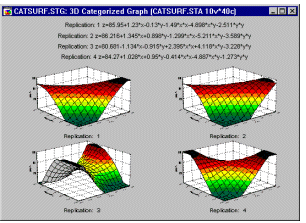
This would give you a graphical indication of the reliability of the results and where (e.g., in which region of the surface) deviations occur.
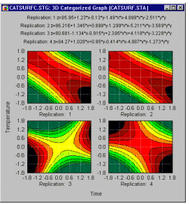
Clearly, the third replication produced a different surface. In replications 1, 2, and 4, the fitted surfaces are very similar to each other. Thus, one should investigate what could have caused this noticeable difference in the third replication of the design.
| To index |
Latin square designs (the term Latin square was first used by Euler, 1782) are used when the factors of interest have more than two levels and you know ahead of time that there are no (or only negligible) interactions between factors. For example, if you wanted to examine the effect of 4 fuel additives on reduction in oxides of nitrogen and had 4 cars and 4 drivers at your disposal, then you could of course run a full 4 x 4 x 4 factorial design, resulting in 64 experimental runs. However, you are not really interested in any (minor) interactions between the fuel additives and drivers, fuel additives and cars, or cars and drivers. You are mostly interested in estimating main effects, in particular the one for the fuel additives factor. At the same time, you want to make sure that the main effects for drivers and cars do not affect (bias) your estimate of the main effect for the fuel additive.
If you labeled the additives with the letters A, B, C, and D, the Latin square design that would allow you to derive unconfounded main effects estimates could be summarized as follows (see also Box, Hunter, and Hunter, 1978, page 263):
| Car | ||||
|---|---|---|---|---|
| Driver | 1 | 2 | 3 | 4 |
| 1 2 3 4 |
A D B C |
B C D A |
D A C B |
C B A D |
The example shown above is actually only one of the three possible arrangements in effect estimates. These "arrangements" are also called Latin square. The example above constitutes a 4 x 4 Latin square; and rather than requiring the 64 runs of the complete factorial, you can complete the study in only 16 runs.
Greco-Latin square. A nice feature of Latin Squares is that they can be superimposed to form what are called Greco-Latin squares (this term was first used by Fisher and Yates, 1934). For example, the following two 3 x 3 Latin squares can be superimposed to form a Greco-Latin square:

In the resultant Greco-Latin square design, you can evaluate the main effects of four 3-level factors (row factor, column factor, Roman letters, Greek letters) in only 9 runs.
Hyper-Greco Latin square. For some numbers of levels, there are more than two possible Latin square arrangements. For example, there are three possible arrangements for 4-level Latin squares. If all three of them are superimposed, you get a Hyper-Greco Latin square design. In that design you can estimate the main effects of all five 4-level factors with only 16 runs in the experiment.
Analyzing the Design
Analyzing Latin square designs is straightforward. Also, plots of means can be produced to aid in the interpretation of results.
Very Large Designs, Random Effects, Unbalanced Nesting
Note that there are several other statistical methods that can also analyze these types of designs; see the section on Methods for Analysis of Variance for details. In particular the Variance Components and Mixed Model ANOVA/ANCOVA chapter discusses very efficient methods for analyzing designs with unbalanced nesting (when the nested factors have different numbers of levels within the levels of the factors in which they are nested), very large nested designs (e.g., with more than 200 levels overall), or hierarchically nested designs (with or without random factors).
| To index |
Applications. Taguchi methods have become increasingly popular in recent years. The documented examples of sizable quality improvements that resulted from implementations of these methods (see, for example, Phadke, 1989; Noori, 1989) have added to the curiosity among American manufacturers. In fact, some of the leading manufacturers in this country have begun to use these methods with usually great success. For example, AT&T is using these methods in the manufacture of very large scale integrated (VLSI) circuits; also, Ford Motor Company has gained significant quality improvements due to these methods (American Supplier Institute, 1984 to 1988). However, as the details of these methods are becoming more widely known, critical appraisals are also beginning to appear (for example, Bhote, 1988; Tribus and Szonyi, 1989).
Overview. Taguchi robust design methods are set apart from traditional quality control procedures (see Quality Control and Process Analysis) and industrial experimentation in various respects. Of particular importance are:
Quality and Loss Functions
What is quality. Taguchi's analysis begins with the question of how to define quality. It is not easy to formulate a simple definition of what constitutes quality; however, when your new car stalls in the middle of a busy intersection -- putting yourself and other motorists at risk -- you know that your car is not of high quality. Put another way, the definition of the inverse of quality is rather straightforward: it is the total loss to you and society due to functional variations and harmful side effects associated with the respective product. Thus, as an operational definition, you can measure quality in terms of this loss, and the greater the quality loss the lower the quality.
Discontinuous (step-shaped) loss function. You can formulate hypotheses about the general nature and shape of the loss function. Assume a specificideal point of highest quality; for example, a perfect car with no quality problems. It is customary in statistical process control (SPC; see also Process Analysis) to define tolerances around the nominal ideal point of the production process. According to the traditional view implied by common SPC methods, as long as you are within the manufacturing tolerances you do not have a problem. Put another way, within the tolerance limits the quality loss is zero; once you move outside the tolerances, the quality loss is declared to be unacceptable. Thus, according to traditional views, the quality loss function is a discontinuous step function: as long as you are within the tolerance limits, quality loss is negligible; when you step outside those tolerances, quality loss becomes unacceptable.
Quadratic loss function. Is the step function implied by common SPC methods a good model of quality loss? Return to the "perfect automobile" example. Is there a difference between a car that, within one year after purchase, has nothing wrong with it, and a car where minor rattles develop, a few fixtures fall off, and the clock in the dashboard breaks (all in-warranty repairs, mind you...)? If you ever bought a new car of the latter kind, you know very well how annoying those admittedly minor quality problems can be. The point here is that it is not realistic to assume that, as you move away from the nominal specification in your production process, the quality loss is zero as long as you stay within the set tolerance limits. Rather, if you are not exactly "on target," then loss will result, for example in terms of customer satisfaction. Moreover, this loss is probably not a linear function of the deviation from nominal specifications, but rather a quadratic function (inverted U). A rattle in one place in your new car is annoying, but you would probably not get too upset about it; add two more rattles, and you might declare the car "junk." Gradual deviations from the nominal specifications do not produce proportional increments in loss, but rather squared increments.
Conclusion: Controlling variability. If, in fact, quality loss is a quadratic function of the deviation from a nominal value, then the goal of your quality improvement efforts should be to minimize the squared deviations or variance of the product around nominal (ideal) specifications, rather than the number of units within specification limits (as is done in traditional SPC procedures).
Signal-to-Noise (S/N) Ratios
Measuring quality loss. Even though you have concluded that the quality loss function is probably quadratic in nature, you still do not know precisely how to measure quality loss. However, you know that whatever measure you decide upon should reflect the quadratic nature of the function.
Signal, noise, and control factors. The product of ideal quality should always respond in exactly the same manner to the signals provided by the user. When you turn the key in the ignition of your car you expect that the starter motor turns and the engine starts. In the ideal-quality car, the starting process would always proceed in exactly the same manner -- for example, after three turns of the starter motor the engine comes to life. If, in response to the same signal (turning the ignition key) there is random variability in this process, then you have less than ideal quality. For example, due to such uncontrollable factors as extreme cold, humidity, engine wear, etc. the engine may sometimes start only after turning over 20 times and finally not start at all. This example illustrates the key principle in measuring quality according to Taguchi: You want to minimize the variability in the product's performance in response to noise factors while maximizing the variability in response to signal factors.
Noise factors are those that are not under the control of the operator of a product. In the car example, those factors include temperature changes, different qualities of gasoline, engine wear, etc. Signal factors are those factors that are set or controlled by the operator of the product to make use of its intended functions (turning the ignition key to start the car).
Finally, the goal of your quality improvement effort is to find the best settings of factors under your control that are involved in the production process, in order to maximize the S/N ratio; thus, the factors in the experiment represent control factors.
S/N ratios. The conclusion of the previous paragraph is that quality can be quantified in terms of the respective product's response to noise factors and signal factors. The ideal product will only respond to the operator's signals and will be unaffected by random noise factors (weather, temperature, humidity, etc.). Therefore, the goal of your quality improvement effort can be stated as attempting to maximize the signal-to-noise (S/N) ratio for the respective product. The S/N ratios described in the following paragraphs have been proposed by Taguchi (1987).
Smaller-the-better. In cases where you want to minimize the occurrences of some undesirable product characteristics, you would compute the following S/N ratio:
Eta = -10 * log10 [(1/n) *  (yi2)] for i = 1 to no. vars
see outer arrays
Here, Eta is the resultant S/N ratio; n is the number of observations on the particular product, and y is the respective characteristic. For example, the number of flaws in the paint on an automobile could be measured as the y variable and analyzed via this S/N ratio. The effect of the signal factors is zero, since zero flaws is the only intended or desired state of the paint on the car. Note how this S/N ratio is an expression of the assumed quadratic nature of the loss function. The factor 10 ensures that this ratio measures the inverse of "bad quality;" the more flaws in the paint, the greater is the sum of the squared number of flaws, and the smaller (i.e., more negative) the S/N ratio. Thus, maximizing this ratio will increase quality.
Nominal-the-best. Here, you have a fixed signal value (nominal value), and the variance around this value can be considered the result of noise factors:
Eta = 10 * log10 (Mean2/Variance)
This signal-to-noise ratio could be used whenever ideal quality is equated with a particular nominal value. For example, the size of piston rings for an automobile engine must be as close to specification as possible to ensure high quality.
Larger-the-better. Examples of this type of engineering problem are fuel economy (miles per gallon) of an automobile, strength of concrete, resistance of shielding materials, etc. The following S/N ratio should be used:
Eta = -10 * log10 [(1/n) *  (1/yi2)] for i = 1 to no. vars
see outer arrays
Signed target. This type of S/N ratio is appropriate when the quality characteristic of interest has an ideal value of 0 (zero), and both positive and negative values of the quality characteristic may occur. For example, the dc offset voltage of a differential operational amplifier may be positive or negative (see Phadke, 1989). The following S/N ratio should be used for these types of problems:
Eta = -10 * log10(s2) for i = 1 to no. vars see outer arrays
where s2 stands for the variance of the quality characteristic across the measurements (variables).Fraction defective. This S/N ratio is useful for minimizing scrap, minimizing the percent of patients who develop side-effects to a drug, etc. Taguchi also refers to the resultant Eta values as Omegas; note that this S/N ratio is identical to the familiar logit transformation (see also Nonlinear Estimation):
Eta = -10 * log10[p/(1-p)]
where
p is the proportion defective
Ordered categories (the accumulation analysis). In some cases, measurements on a quality characteristic can only be obtained in terms of categorical judgments. For example, consumers may rate a product as excellent, good, average, or below average. In that case, you would attempt to maximize the number of excellent or good ratings. Typically, the results of an accumulation analysis are summarized graphically in a stacked bar plot.
Orthogonal Arrays
The third aspect of Taguchi robust design methods is the one most similar to traditional techniques. Taguchi has developed a system of tabulated designs (arrays) that allow for the maximum number of main effects to be estimated in an unbiased (orthogonal) manner, with a minimum number of runs in the experiment. Latin square designs, 2**(k-p) designs (Plackett-Burman designs, in particular), and Box-Behnken designs main are also aimed at accomplishing this goal. In fact, many of the standard orthogonal arrays tabulated by Taguchi are identical to fractional two-level factorials, Plackett-Burman designs, Box-Behnken designs, Latin square, Greco-Latin squares, etc.
Analyzing Designs
Most analyses of robust design experiments amount to a standard ANOVA of the respective S/N ratios, ignoring two-way or higher-order interactions. However, when estimating error variances, one customarily pools together main effects of negligible size.
Analyzing S/N ratios in standard designs. It should be noted at this point that, of course, all of the designs discussed up to this point (e.g., 2**(k-p), 3**(k-p), mixed 2 and 3 level factorials, Latin squares, central composite designs) can be used to analyze S/N ratios that you computed. In fact, the many additional diagnostic plots and other options available for those designs (e.g., estimation of quadratic components, etc.) may prove very useful when analyzing the variability (S/N ratios) in the production process.
Plot of means. A visual summary of the experiment is the plot of the average Eta (S/N ratio) by factor levels. In this plot, the optimum setting (i.e., largest S/N ratio) for each factor can easily be identified.
Verification experiments. For prediction purposes, you can compute the expected S/N ratio given a user-defined combination of settings of factors (ignoring factors that were pooled into the error term). These predicted S/N ratios can then be used in a verification experiment, where the engineer actually sets the machine accordingly and compares the resultant observed S/N ratio with the predicted S/N ratio from the experiment. If major deviations occur, one must conclude that the simple main effect model is not appropriate.
In those cases, Taguchi (1987) recommends transforming the dependent variable to accomplish additivity of factors, that is, to "make" the main effects model fit. Phadke (1989, Chapter 6) also discusses in detail methods for achieving additivity of factors.
Accumulation Analysis
When analyzing ordered categorical data, ANOVA is not appropriate. Rather, you produce a cumulative plot of the number of observations in a particular category. For each level of each factor, you plot the cumulative proportion of the number of defectives. Thus, this graph provides valuable information concerning the distribution of the categorical counts across the different factor settings.
Summary
To briefly summarize, when using Taguchi methods you first need to determine the design or control factors that can be set by the designer or engineer. Those are the factors in the experiment for which you will try different levels. Next, you decide to select an appropriate orthogonal array for the experiment. Next, you need to decide on how to measure the quality characteristic of interest. Remember that most S/N ratios require that multiple measurements are taken in each run of the experiment; for example, the variability around the nominal value cannot otherwise be assessed. Finally, you conduct the experiment and identify the factors that most strongly affect the chosen S/N ratio, and you reset your machine or production process accordingly.
| To index |
Special issues arise when analyzing mixtures of components that must sum to a constant. For example, if you wanted to optimize the taste of a fruit-punch, consisting of the juices of 5 fruits, then the sum of the proportions of all juices in each mixture must be 100%. Thus, the task of optimizing mixtures commonly occurs in food-processing, refining, or the manufacturing of chemicals. A number of designs have been developed to address specifically the analysis and modeling of mixtures (see, for example, Cornell, 1990a, 1990b; Cornell and Khuri, 1987; Deming and Morgan, 1993; Montgomery, 1991).
Triangular Coordinates
The common manner in which mixture proportions can be summarized is via triangular (ternary) graphs. For example, suppose you have a mixture that consists of 3 components A, B, and C. Any mixture of the three components can be summarized by a point in the triangular coordinate system defined by the three variables.
For example, take the following 6 different mixtures of the 3 components.
| A | B | C |
|---|---|---|
| 1 0 0 0.5 0.5 0 |
0 1 0 0.5 0 0.5 |
0 0 1 0 0.5 0.5 |
The sum for each mixture is 1.0, so the values for the components in each mixture can be interpreted as proportions. If you graph these data in a regular 3D scatterplot, it becomes apparent that the points form a triangle in the 3D space. Only the points inside the triangle where the sum of the component values is equal to 1 are valid mixtures. Therefore, one can simply plot only the triangle to summarize the component values (proportions) for each mixture.
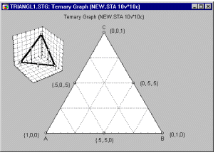
To read-off the coordinates of a point in the triangular graph, you would simply "drop" a line from each respective vertex to the side of the triangle below.
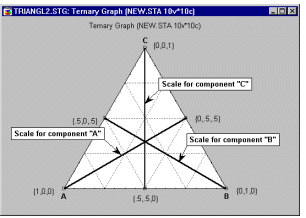
At the vertex for the particular factor, there is a pure blend, that is, one that only contains the respective component. Thus, the coordinates for the vertex point is 1 (or 100%, or however else the mixtures are scaled) for the respective component, and 0 (zero) for all other components. At the side opposite to the respective vertex, the value for the respective component is 0 (zero), and .5 (or 50%, etc.) for the other components.
Triangular Surfaces and Contours
One can now add to the triangle a fourth dimension, that is perpendicular to the first three. Using that dimension, one could plot the values for a dependent variable, or function (surface) that was fit to the dependent variable. Note that the response surface can either be shown in 3D, where the predicted response (Taste rating) is indicated by the distance of the surface from the triangular plane, or it can be indicated in a contour plot where the contours of constant height are plotted on the 2D triangle.
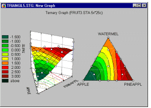
It should be mentioned at this point that you can produce categorized ternary graphs. These are very useful, because they allow you to fit to a dependent variable (e.g., Taste) a response surface, for different levels of a fourth component.
The Canonical Form of Mixture Polynomials
Fitting a response surface to mixture data is, in principle, done in the same manner as fitting surfaces to, for example, data from central composite designs. However, there is the issue that mixture data are constrained, that is, the sum of all component values must be constant.
Consider the simple case of two factors A and B. One may want to fit the simple linear model:
y = b0 + bA*xA + bB*xB
Here y stands for the dependent variable values, bA and bB stand for the regression coefficients, xA and xB stand for the values of the factors. Suppose that xA and xB must sum to 1; you can multiple b0 by 1=(xA + xB):
y = (b0*xA + b0*xB) + bA*xA + bB*xB
or:
y = b'A*xA + b'B*xB
where b'A = b0 + bA and b'B = b0 + bB. Thus, the estimation of this model comes down to fitting a no- intercept multiple regression model. (See also Multiple Regression, for details concerning multiple regression.)
Common Models for Mixture Data
The quadratic and cubic model can be similarly simplified (as illustrated for the simple linear model above), yielding four standard models that are customarily fit to the mixture data. Here are the formulas for the 3-variable case for those models (see Cornell, 1990, for additional details).
Linear model:
y = b1*x1 + b2*x2 + b3*x3
Quadratic model:
y = b1*x1 + b2*x2 + b3*x3 + b12*x1*x2 + b13*x1*x3 + b23*x2*x3
Special cubic model:
y = b1*x1 + b2*x2 + b3*x3 + b12*x1*x2 + b13*x1*x3 + b23*x2*x3 + b123*x1*x2*x3
Full cubic model:
y = b1*x1 + b2*x2 + b3*x3 + b12*x1*x2 + b13*x1*x3 + b23*x2*x3 + d12*x1*x2*(x1 - x2) + d13*x1*x3*(x1 - x3) + d23*x2*x3*(x2 - x3) + b123*x1*x2*x3
(Note that the dij's are also parameters of the model.)
Standard Designs for Mixture Experiments
Two different types of standard designs are commonly used for experiments with mixtures. Both of them will evaluate the triangular response surface at the vertices (i.e., the corners of the triangle) and the centroids (sides of the triangle). Sometimes, those designs are enhanced with additional interior points.
Simplex-lattice designs. In this arrangement of design points, m+1 equally spaced proportions are tested for each factor or component in the model:
xi = 0, 1/m, 2/m, ..., 1 i = 1,2,...,q
and all combinations of factor levels are tested. The resulting design is called a {q,m} simplex lattice design. For example, a {q=3, m=2} simplex lattice design will include the following mixtures:
| A | B | C |
|---|---|---|
| 1 0 0 .5 .5 0 |
0 1 0 .5 0 .5 |
0 0 1 0 .5 .5 |
A {q=3,m=3} simplex lattice design will include the points:
| A | B | C |
|---|---|---|
| 1 0 0 1/3 1/3 0 2/3 2/3 0 1/3 |
0 1 0 2/3 0 1/3 1/3 0 2/3 1/3 |
0 0 1 0 2/3 2/3 0 1/3 1/3 1/3 |
Simplex-centroid designs. An alternative arrangement of settings introduced by Scheff� (1963) is the so-called simplex-centroid design. Here the design points correspond to all permutations of the pure blends (e.g., 1 0 0; 0 1 0; 0 0 1), the permutations of the binary blends (� � 0; � 0 �; 0 � �), the permutations of the blends involving three components, and so on. For example, for 3 factors the simplex centroid design consists of the points:
| A | B | C |
|---|---|---|
| 1 0 0 1/2 1/2 0 1/3 |
0 1 0 1/2 0 1/2 1/3 |
0 0 1 0 1/2 1/2 1/3 |
Adding interior points. These designs are sometimes augmented with interior points (see Khuri and Cornell, 1987, page 343; Mason, Gunst, Hess; 1989; page 230). For example, for 3 factors one could add the interior points:
| A | B | C |
|---|---|---|
| 2/3 1/6 1/6 |
1/6 2/3 1/6 |
1/6 1/6 2/3 |
If you plot these points in a scatterplot with triangular coordinates; one can see how these designs evenly cover the experimental region defined by the triangle.
Lower Constraints
The designs described above all require vertex points, that is, pure blends consisting of only one ingredient. In practice, those points may often not be valid, that is, pure blends cannot be produced because of cost or other constraints. For example, suppose you wanted to study the effect of a food- additive on the taste of the fruit-punch. The additional ingredient may only be varied within small limits, for example, it may not exceed a certain percentage of the total. Clearly, a fruit punch that is a pure blend, consisting only of the additive, would not be a fruit punch at all, or worse, may be toxic. These types of constraints are very common in many applications of mixture experiments.
Let us consider a 3-component example, where component A is constrained so that xA .3. The total of the 3-component mixture must be equal to 1. This constraint can be visualized in a triangular graph by a line at the triangular coordinate for xA=.3, that is, a line that is parallel to the triangle's edge opposite to the A vertex point.
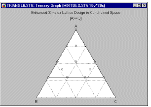
One can now construct the design as before, except that one side of the triangle is defined by the constraint. Later, in the analysis, one can review the parameter estimates for the so-called pseudo-components, treating the constrained triangle as if it were a full triangle.
Multiple constraints. Multiple lower constraints can be treated analogously, that is, you can construct the sub-triangle within the full triangle, and then place the design points in that sub-triangle according to the chosen design.
Upper and Lower Constraints
When there are both upper and lower constraints (as is often the case in experiments involving mixtures), then the standard simplex-lattice and simplex-centroid designs can no longer be constructed, because the subregion defined by the constraints is no longer a triangle. There is a general algorithm for finding the vertex and centroid points for such constrained designs.
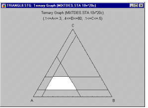
Note that you can still analyze such designs by fitting the standard models to the data.
Analyzing Mixture Experiments
The analysis of mixture experiments amounts to a multiple regression with the intercept set to zero. As explained earlier, the mixture constraint -- that the sum of all components must be constant -- can be accommodated by fitting multiple regression models that do not include an intercept term. If you are not familiar with multiple regression, you may want to review at this point Multiple Regression.
The specific models that are usually considered were described earlier. To summarize, one fits to the dependent variable response surfaces of increasing complexity, that is, starting with the linear model, then the quadratic model, special cubic model, and full cubic model. Shown below is a table with the number of terms or parameters in each model, for a selected number of components (see also Table 4, Cornell, 1990):
| Model (Degree of Polynomial) | ||||
|---|---|---|---|---|
| No. of Comp. |
Linear |
Quadr. |
Special Cubic |
Full Cubic |
| 2 3 4 5 6 7 8 |
2 3 4 5 6 7 8 |
3 6 10 15 21 28 36 |
-- 7 14 25 41 63 92 |
-- 10 20 35 56 84 120 |
Analysis of Variance
To decide which of the models of increasing complexity provides a sufficiently good fit to the observed data, one usually compares the models in a hierarchical, stepwise fashion. For example, consider a 3- component mixture to which the full cubic model was fitted.
| ANOVA; Var.:DV (mixt4.sta) | ||||||||||
|---|---|---|---|---|---|---|---|---|---|---|
| 3 Factor mixture design; Mixture total=1., 14 Runs Sequential fit of models of increasing complexity |
||||||||||
| Model |
SS Effect |
df Effect |
MS Effect |
SS Error |
df Error |
MS Error |
F |
p |
R-sqr |
R-sqr Adj. |
| Linear Quadratic Special Cubic Cubic Total Adjusted |
44.755 30.558 .719 8.229 91.627 |
2 3 1 3 13 |
22.378 10.186 .719 2.743 7.048 |
46.872 16.314 15.596 7.367 |
11 8 7 4 |
4.2611 2.0393 2.2279 1.8417 |
5.2516 4.9949 .3225 1.4893 |
.0251 .0307 .5878 .3452 |
.4884 .8220 .8298 .9196 |
.3954 .7107 .6839 .7387 |
First, the linear model was fit to the data. Even though this model has 3 parameters, one for each component, this model has only 2 degrees of freedom. This is because of the overall mixture constraint, that the sum of all component values is constant. The simultaneous test for all parameters of this model is statistically significant (F(2,11)=5.25; p<.05). The addition of the 3 quadratic model parameters (b12*x1*x2, b13*x1*x3, b23*x2*x3) further significantly improves the fit of the model (F(3,8)=4.99; p<.05). However, adding the parameters for the special cubic and cubic models does not significantly improve the fit of the surface. Thus one could conclude that the quadratic model provides an adequate fit to the data (of course, pending further examination of the residuals for outliers, etc.).
R-square. The R-square value can be interpreted as the proportion of variability around the mean for the dependent variable, that can be accounted for by the respective model. (Note that for non- intercept models, some multiple regression programs will only compute the R-square value pertaining to the proportion of variance around 0 (zero) accounted for by the independent variables; for more information, see Kvalseth, 1985; Okunade, Chang, and Evans, 1993.)
Pure error and lack of fit. The usefulness of the estimate of pure error for assessing the overall lack of fit was discussed in the context of central composite designs. If some runs in the design were replicated, then one can compute an estimate of error variability based only on the variability between replicated runs. This variability provides a good indication of the unreliability in the measurements, independent of the model that was fit to the data, since it is based on identical factor settings (or blends in this case). One can test the residual variability after fitting the current model against this estimate of pure error. If this test is statistically significant, that is, if the residual variability is significantly larger than the pure error variability, then one can conclude that, most likely, there are additional significant differences between blends that cannot be accounted for by the current model. Thus, there may be an overall lack of fit of the current model. In that case, try a more complex model, perhaps by only adding individual terms of the next higher-order model (e.g., only the b13*x1*x3 to the linear model).
Parameter Estimates
Usually, after fitting a particular model, one would next review the parameter estimates. Remember that the linear terms in mixture models are constrained, that is, the sum of the components must be constant. Hence, independent statistical significance tests for the linear components cannot be performed.
Pseudo-Components
To allow for scale-independent comparisons of the parameter estimates, during the analysis, the component settings are customarily recoded to so-called pseudo-components so that (see also Cornell, 1993, Chapter 3):
x'i = (xi-Li)/(Total-L)
Here, x'i stands for the i'th pseudo-component, xi stands for the original component value, Li stands for the lower constraint (limit) for the i'th component, L stands for the sum of all lower constraints (limits) for all components in the design, and Total is the mixture total.
The issue of lower constraints was also discussed earlier in this section. If the design is a standard simplex-lattice or simplex-centroid design (see above), then this transformation amounts to a rescaling of factors so as to form a sub-triangle (sub-simplex) as defined by the lower constraints. However, you can compute the parameter estimates based on the original (untransformed) metric of the components in the experiment. If you want to use the fitted parameter values for prediction purposes (i.e., to predict dependent variable values), then the parameters for the untransformed components are often more convenient to use. Note that the results dialog for mixture experiments contains options to make predictions for the dependent variable for user-defined values of the components, in their original metric.
Graph Options
Surface and contour plots. The respective fitted model can be visualized in triangular surface plots or contour plots, which, optionally, can also include the respective fitted function.
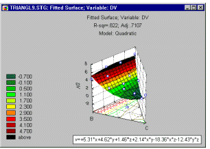
Note that the fitted function displayed in the surface and contour plots always pertains to the parameter estimates for the pseudo-components.
Categorized surface plots. If your design involves replications (and the replications are coded in your data file), then you can use 3D Ternary Plots to look at the respective fit, replication by replication.
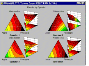
Of course, if you have other categorical variables in your study (e.g., operator or experimenter; machine, etc.) you can also categorize the 3D surface plot by those variables.
Trace plots. One aid for interpreting the triangular response surface is the so-called trace plot. Suppose you looked at the contour plot of the response surface for three components. Then, determine a reference blend for two of the components, for example, hold the values for A and B at 1/3 each. Keeping the relative proportions of A and B constant (i.e., equal proportions in this case), you can then plot the estimated response (values for the dependent variable) for different values of C.
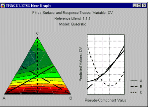
If the reference blend for A and B is 1:1, then the resulting line or response trace is the axis for factor C; that is, the line from the C vertex point connecting with the opposite side of the triangle at a right angle. However, trace plots for other reference blends can also be produced. Typically, the trace plot contains the traces for all components, given the current reference blend.
Residual plots. Finally, it is important, after deciding on a model, to review the prediction residuals, in order to identify outliers or regions of misfit-fit. In addition, one should review the standard normal probability plot of residuals and the scatterplot of observed versus predicted values. Remember that the multiple regression analysis (i.e., the process of fitting the surface) assumes that the residuals are normally distributed, and one should carefully review the residuals for any apparent outliers.
| To index |
Overview
As mentioned in the context of mixture designs, it often happens in real-world studies that the experimental region of interest is constrained, that is, that not all factors settings can be combined with all settings for the other factors in the study. There is an algorithm suggested by Piepel (1988) and Snee (1985) for finding the vertices and centroids for such constrained regions.
Designs for Constrained Experimental Regions
When in an experiment with many factors, there are constraints concerning the possible values of those factors and their combinations, it is not clear how to proceed. A reasonable approach is to include in the experiments runs at the extreme vertex points and centroid points of the constrained region, which should usually provide good coverage of the constrained experimental region (e.g., see Piepel, 1988; Snee, 1975). In fact, the mixture designs reviewed in the previous section provide examples for such designs, since they are typically constructed to include the vertex and centroid points of the constrained region that consists of a triangle (simplex).
Linear Constraints
One general way in which one can summarize most constraints that occur in real world experimentation is in terms of a linear equation (see Piepel, 1988):
A1x1 + A2x2 + ... + Aqxq + A0  0
0
Here, A0, .., Aq are the parameters for the linear constraint on the q factors, and x1,.., xq stands for the factor values (levels) for the q factors. This general formula can accommodate even very complex constraints. For example, suppose that in a two-factor experiment the first factor must always be set at least twice as high as the second, that is, x1  2*x2. This simple constraint can be rewritten as x1-2*x2
  0. The ratio constraint 2*x1 /x2
 1 can be rewritten as 2*x1 - x2
  0, and so on.
The problem of multiple upper and lower constraints on the component values in mixtures was discussed earlier, in the context of mixture experiments. For example, suppose in a three-component mixture of fruit juices, the upper and lower constraints on the components are (see example 3.2, in Cornell 1993):
40%  Watermelon (x1)
  80%
80%
10%  Pineapple (x2)
  50%
50%
10%  Orange (x3)
  30%
30%
These constraints can be rewritten as linear constraints into the form:
| Watermelon: |
x1-40 0 0-x1+80  0 0 |
| Pineapple: |
x2-10 0 0-x2+50  0 0 |
| Orange: |
x3-10 0 0-x3+30  0 0 |
Thus, the problem of finding design points for mixture experiments with components with multiple upper and lower constraints is only a special case of general linear constraints.
The Piepel & Snee Algorithm
For the special case of constrained mixtures, algorithms such as the XVERT algorithm (see, for example, Cornell, 1990) are often used to find the vertex and centroid points of the constrained region (inside the triangle of three components, tetrahedron of four components, etc.). The general algorithm proposed by Piepel (1988) and Snee (1979) for finding vertices and centroids can be applied to mixtures as well as non-mixtures. The general approach of this algorithm is described in detail by Snee (1979).
Specifically, it will consider one-by-one each constraint, written as a linear equation as described above. Each constraint represents a line (or plane) through the experimental region. For each successive constraint the you will evaluate whether or not the current (new) constraint crosses into the current valid region of the design. If so, new vertices will be computed which define the new valid experimental region, updated for the most recent constraint. It will then check whether or not any of the previously processed constraints have become redundant, that is, define lines or planes in the experimental region that are now entirely outside the valid region. After all constraints have been processed, it will then compute the centroids for the sides of the constrained region (of the order requested by the user). For the two-dimensional (two-factor) case, one can easily recreate this process by simply drawing lines through the experimental region, one for each constraint; what is left is the valid experimental region.
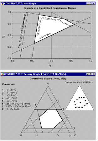
For more information, see Piepel (1988) or Snee (1979).
Choosing Points for the Experiment
Once the vertices and centroids have been computed, you may face the problem of having to select a subset of points for the experiment. If each experimental run is costly, then it may not be feasible to simply run all vertex and centroid points. In particular, when there are many factors and constraints, then the number of centroids can quickly get very large.
If you are screening a large number of factors, and are not interested in non-linear effects, then choosing the vertex points only will usually yield good coverage of the experimental region. To increase statistical power (to increase the degrees of freedom for the ANOVA error term), you may also want to include a few runs with the factors set at the overall centroid of the constrained region.
If you are considering a number of different models that you might fit once the data have been collected, then you may want to use the D- and A-optimal design options. Those options will help you select the design points that will extract the maximum amount of information from the constrained experimental region, given your models.
Analyzing Designs for Constrained Surfaces and Mixtures
As mentioned in the section on central composite designs and mixture designs, once the constrained design points have been chosen for the final experiment, and the data for the dependent variables of interest have been collected, the analysis of these designs can proceed in the standard manner.
For example, Cornell (1990, page 68) describes an experiment of three plasticizers, and their effect on resultant vinyl thickness (for automobile seat covers). The constraints for the three plasticizers components x1, x2, and x3 are:
.409  x1
x1  .849
.849
.000  x2
x2  .252
.252
.151  x3
x3  .274
.274
(Note that these values are already rescaled, so that the total for each mixture must be equal to 1.) The vertex and centroid points generated are:
| x1 | x2 | x3 |
|---|---|---|
| .8490 .7260 .4740 .5970 .6615 .7875 .6000 .5355 .7230 |
.0000 .0000 .2520 .2520 .1260 .0000 .1260 .2520 .1260 |
.1510 .2740 .2740 .1510 .2125 .2125 .2740 .2125 .1510 |
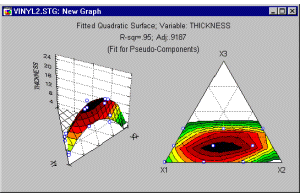
| To index |
Overview
In the sections on standard factorial designs (see 2**(k-p) Fractional Factorial Designs and 3**(k-p), Box Behnken, and Mixed 2 and 3 Level Factorial Designs) and Central Composite Designs, the property of orthogonality of factor effects was discussed. In short, when the factor level settings for two factors in an experiment are uncorrelated, that is, when they are varied independently of each other, then they are said to be orthogonal to each other. (If you are familiar with matrix and vector algebra, two column vectors X1 and X2 in the design matrix are orthogonal if X1'*X2= 0). Intuitively, it should be clear that one can extract the maximum amount of information regarding a dependent variable from the experimental region (the region defined by the settings of the factor levels), if all factor effects are orthogonal to each other. Conversely, suppose one ran a four-run experiment for two factors as follows:
| x1 | x2 | |
|---|---|---|
| Run 1 Run 2 Run 3 Run 4 |
1 1 -1 -1 |
1 1 -1 -1 |
Now the columns of factor settings for X1 and X2 are identical to each other (their correlation is 1), and there is no way in the results to distinguish between the main effect for X1 and X2.
The D- and A-optimal design procedures provide various options to select from a list of valid (candidate) points (i.e., combinations of factor settings) those points that will extract the maximum amount of information from the experimental region, given the respective model that you expect to fit to the data. You need to supply the list of candidate points, for example the vertex and centroid points computed by the Designs for constrained surface and mixtures option, specify the type of model you expect to fit to the data, and the number of runs for the experiment. It will then construct a design with the desired number of cases, that will provide as much orthogonality between the columns of the design matrix as possible.
The reasoning behind D- and A-optimality is discussed, for example, in Box and Draper (1987, Chapter 14). The different algorithms used for searching for optimal designs are described in Dykstra (1971), Galil and Kiefer (1980), and Mitchell (1974a, 1974b). A detailed comparison study of the different algorithms is discussed in Cook and Nachtsheim (1980).
Basic Ideas
A technical discussion of the reasoning (and limitations) of D- and A-optimal designs is beyond the scope of this introduction. However, the general ideas are fairly straight-forward. Consider again the simple two-factor experiment in four runs.
| x1 | x2 | |
|---|---|---|
| Run 1 Run 2 Run 3 Run 4 |
1 1 -1 -1 |
1 1 -1 -1 |
As mentioned above, this design, of course, does not allow one to test, independently, the statistical significance of the two variables' contribution to the prediction of the dependent variable. If you computed the correlation matrix for the two variables, they would correlate at 1:
| x1 | x2 | |
|---|---|---|
| x1 x2 |
1.0 1.0 | 1.0 1.0 |
Normally, one would run this experiment so that the two factors are varied independently of each other:
| x1 | x2 | |
|---|---|---|
| Run 1 Run 2 Run 3 Run 4 |
1 1 -1 -1 |
1 -1 1 -1 |
Now the two variables are uncorrelated, that is, the correlation matrix for the two factors is:
| x1 | x2 | |
|---|---|---|
| x1 x2 |
1.0 0.0 | 0.0 1.0 |
Another term that is customarily used in this context is that the two factors are orthogonal. Technically, if the sum of the products of the elements of two columns (vectors) in the design (design matrix) is equal to 0 (zero), then the two columns are orthogonal.
The determinant of the design matrix. The determinant D of a square matrix (like the 2-by-2 correlation matrices shown above) is a specific numerical value, that reflects the amount of independence or redundancy between the columns and rows of the matrix. For the 2-by-2 case, it is simply computed as the product of the diagonal elements minus the off-diagonal elements of the matrix (for larger matrices the computations are more complex). For example, for the two matrices shown above, the determinant D is:
| D1 = |
|1.0 1.0| |1.0 1.0| |
= 1*1 - 1*1 = 0 |
| D2 = |
|1.0 0.0| |0.0 1.0| |
= 1*1 - 0*0 = 1 |
Thus, the determinant for the first matrix computed from completely redundant factor settings is equal to 0. The determinant for the second matrix, when the factors are orthogonal, is equal to 1.
D-optimal designs. This basic relationship extends to larger design matrices, that is, the more redundant the vectors (columns) of the design matrix, the closer to 0 (zero) is the determinant of the correlation matrix for those vectors; the more independent the columns, the larger is the determinant of that matrix. Thus, finding a design matrix that maximizes the determinant D of this matrix means finding a design where the factor effects are maximally independent of each other. This criterion for selecting a design is called the D-optimality criterion.
Matrix notation. Actually, the computations are commonly not performed on the correlation matrix of vectors, but on the simple cross-product matrix. In matrix notation, if the design matrix is denoted by X, then the quantity of interest here is the determinant of X'X (X- transposed times X). Thus, the search for D-optimal designs aims to maximize |X'X|, where the vertical lines (|..|) indicate the determinant.
A-optimal designs. Looking back at the computations for the determinant, another way to look at the issue of independence is to maximize the diagonal elements of the X'X matrix, while minimizing the off-diagonal elements. The so-called trace criterion or A-optimality criterion expresses this idea. Technically, the A-criterion is defined as:
A = trace(X'X)-1
where trace stands for the sum of the diagonal elements (of the (X'X)-1 matrix).
The information function. It should be mentioned at this point that D-optimal designs minimize the expected prediction error for the dependent variable, that is, those designs will maximize the precision of prediction, and thus the information (which is defined as the inverse of the error) that is extracted from the experimental region of interest.
Measuring Design Efficiency
A number of standard measures have been proposed to summarize the efficiency of a design.
D-efficiency. This measure is related to the D-optimality criterion:
D-efficiency = 100 * (|X'X|1/p/N)
Here, p is the number of factor effects in the design (columns in X), and N is the number of requested runs. This measure can be interpreted as the relative number of runs (in percent) that would be required by an orthogonal design to achieve the same value of the determinant |X'X|. However, remember that an orthogonal design may not be possible in many cases, that is, it is only a theoretical "yard-stick." Therefore, you should use this measure rather as a relative indicator of efficiency, to compare other designs of the same size, and constructed from the same design points candidate list. Also note that this measure is only meaningful (and will only be reported) if you chose to recode the factor settings in the design (i.e., the factor settings for the design points in the candidate list), so that they have a minimum of -1 and a maximum of +1.
A-efficiency. This measure is related to the A-optimality criterion:
A-efficiency = 100 * p/trace(N*(X'X)-1)
Here, p stands for the number of factor effects in the design, N is the number of requested runs, and trace stands for the sum of the diagonal elements (of (N*(X'X)-1) ). This measure can be interpreted as the relative number of runs (in percent) that would be required by an orthogonal design to achieve the same value of the trace of (X'X)-1. However, again you should use this measure as a relative indicator of efficiency, to compare other designs of the same size and constructed from the same design points candidate list; also this measure is only meaningful if you chose to recode the factor settings in the design to the -1 to +1 range.
G-efficiency. This measure is computed as:
G-efficiency = 100 * square root(p/N)/ M
M
Again, p stands for the number of factor effects in the design and N is the number of requested runs;  M (sigmaM) stands for the maximum standard error for prediction across the list of candidate points. This measure is related to the so-called G- optimality criterion; G-optimal designs are defined as those that will minimize the maximum value of the standard error of the predicted response.
Constructing Optimal Designs
The optimal design facilities will "search for" optimal designs, given a list of "candidate points." Put another way, given a list of points that specifies which regions of the design are valid or feasible, and given a user-specified number of runs for the final experiment, it will select points to optimize the respective criterion. This "searching for" the best design is not an exact method, but rather an algorithmic procedure that employs certain search strategies to find the best design (according to the respective optimality criterion).
The search procedures or algorithms that have been proposed are described below (for a review and detailed comparison, see Cook and Nachtsheim, 1980). They are reviewed here in the order of speed, that is, the Sequential or Dykstra method is the fastest method, but often most likely to fail, that is, to yield a design that is not optimal (e.g., only locally optimal; this issue will be discussed shortly).
Sequential or Dykstra method. This algorithm is due to Dykstra (1971). Starting with an empty design, it will search through the candidate list of points, and choose in each step the one that maximizes the chosen criterion. There are no iterations involved, they will simply pick the requested number of points sequentially. Thus, this method is the fastest of the ones discussed. Also, by default, this method is used to construct the initial designs for the remaining methods.
Simple exchange (Wynn-Mitchell) method. This algorithm is usually attributed to Mitchell and Miller (1970) and Wynn (1972). The method starts with an initial design of the requested size (by default constructed via the sequential search algorithm described above). In each iteration, one point (run) in the design will be dropped from the design and another added from the list of candidate points. The choice of points to be dropped or added is sequential, that is, at each step the point that contributes least with respect to the chosen optimality criterion (D or A) is dropped from the design; then the algorithm chooses a point from the candidate list so as to optimize the respective criterion. The algorithm stops when no further improvement is achieved with additional exchanges.
DETMAX algorithm (exchange with excursions). This algorithm, due to Mitchell (1974b), is probably the best known and most widely used optimal design search algorithm. Like the simple exchange method, first an initial design is constructed (by default, via the sequential search algorithm described above). The search begins with a simple exchange as described above. However, if the respective criterion (D or A) does not improve, the algorithm will undertake excursions. Specifically, the algorithm will add or subtract more than one point at a time, so that, during the search, the number of points in the design may vary between ND+ Nexcursion and ND- Nexcursion, where ND is the requested design size, and Nexcursion refers to the maximum allowable excursion, as specified by the user. The iterations will stop when the chosen criterion (D or A) no longer improves within the maximum excursion.
Modified Fedorov (simultaneous switching). This algorithm represents a modification (Cook and Nachtsheim, 1980) of the basic Fedorov algorithm described below. It also begins with an initial design of the requested size (by default constructed via the sequential search algorithm). In each iteration, the algorithm will exchange each point in the design with one chosen from the candidate list, so as to optimize the design according to the chosen criterion (D or A). Unlike the simple exchange algorithm described above, the exchange is not sequential, but simultaneous. Thus, in each iteration each point in the design is compared with each point in the candidate list, and the exchange is made for the pair that optimizes the design. The algorithm terminates when there are no further improvements in the respective optimality criterion.
Fedorov (simultaneous switching). This is the original simultaneous switching method proposed by Fedorov (see Cook and Nachtsheim, 1980). The difference between this procedure and the one described above (modified Fedorov) is that in each iteration only a single exchange is performed, that is, in each iteration all possible pairs of points in the design and those in the candidate list are evaluated. The algorithm will then exchange the pair that optimizes the design (with regard to the chosen criterion). Thus, it is easy to see that this algorithm potentially can be somewhat slow, since in each iteration ND*NC comparisons are performed, in order to exchange a single point.
General Recommendations
If you think about the basic strategies represented by the different algorithms described above, it should be clear that there are usually no exact solutions to the optimal design problem. Specifically, the determinant of the X'X matrix (and trace of its inverse) are complex functions of the list of candidate points. In particular, there are usually several "local minima" with regard to the chosen optimality criterion; for example, at any point during the search a design may appear optimal unless you simultaneously discard half of the points in the design and choose certain other points from the candidate list; but, if you only exchange individual points or only a few points (via DETMAX), then no improvement occurs.
Therefore, it is important to try a number of different initial designs and algorithms. If after repeating the optimization several times with random starts the same, or very similar, final optimal design results, then you can be reasonably sure that you are not "caught" in a local minimum or maximum.
Also, the methods described above vary greatly with regard to their ability to get "trapped" in local minima or maxima. As a general rule, the slower the algorithm (i.e., the further down on the list of algorithms described above), the more likely is the algorithm to yield a truly optimal design. However, note that the modified Fedorov algorithm will practically perform just as well as the unmodified algorithm (see Cook and Nachtsheim, 1980); therefore, if time is not a consideration, we recommend the modified Fedorov algorithm as the best method to use.
D-optimality and A-optimality. For computational reasons (see Galil and Kiefer, 1980), updating the trace of a matrix (for the A-optimality criterion) is much slower than updating the determinant (for D-optimality). Thus, when you choose the A-optimality criterion, the computations may require significantly more time as compared to the D-optimality criterion. Since in practice, there are many other factors that will affect the quality of an experiment (e.g., the measurement reliability for the dependent variable), we generally recommend that you use the D optimality criterion. However, in difficult design situations, for example, when there appear to be many local maxima for the D criterion, and repeated trials yield very different results, you may want to run several optimization trials using the A criterion to learn more about the different types of designs that are possible.
Avoiding Matrix Singularity
It may happen during the search process that it cannot compute the inverse of the X'X matrix (for A-optimality), or that the determinant of the matrix becomes almost 0 (zero). At that point, the search can usually not continue. To avoid this situation, perform the optimization based on an augmented X'X matrix:
X'Xaugmented = X'X +  *(X0'X0/N0)
where X0 stands for the design matrix constructed from the list of all N0 candidate points, and  (alpha) is a user-defined small constant. Thus, you can turn off this feature by setting
  to 0 (zero).
"Repairing" Designs
The optimal design features can be used to "repair" designs. For example, suppose you ran an orthogonal design, but some data were lost (e.g., due to equipment malfunction), and now some effects of interest can no longer be estimated. You could of course make up the lost runs, but suppose you do not have the resources to redo them all. In that case, you can set up the list of candidate points from among all valid points for the experimental region, add to that list all the points that you have already run, and instruct it to always force those points into the final design (and never to drop them out; you can mark points in the candidate list for such forced inclusion). It will then only consider to exclude those points from the design that you did not actually run. In this manner you can, for example, find the best single run to add to an existing experiment, that would optimize the respective criterion.
Constrained Experimental Regions and Optimal Design
A typical application of the optimal design features is to situations when the experimental region of interest is constrained. As described earlier in this section, there are facilities for finding vertex and centroid points for linearly constrained regions and mixtures. Those points can then be submitted as the candidate list for constructing an optimal design of a particular size for a particular model. Thus, these two facilities combined provide a very powerful tool to cope with the difficult design situation when the design region of interest is subject to complex constraints, and one wants to fit particular models with the least number of runs.
| To index |
The following sections introduce several analysis techniques. The sections describe Response/desirability profiling, conducting Residual analyses, and performing Box-Cox transformations of the dependent variable.
See also ANOVA/MANOVA, Methods for Analysis of Variance, and Variance Components and Mixed Model ANOVA/ANCOVA.
Profiling Predicted Responses and Response Desirability
Basic Idea. A typical problem in product development is to find a set of conditions, or levels of the input variables, that produces the most desirable product in terms of its characteristics, or responses on the output variables. The procedures used to solve this problem generally involve two steps: (1) predicting responses on the dependent, or Y variables, by fitting the observed responses using an equation based on the levels of the independent, or X variables, and (2) finding the levels of the X variables which simultaneously produce the most desirable predicted responses on the Y variables. Derringer and Suich (1980) give, as an example of these procedures, the problem of finding the most desirable tire tread compound. There are a number of Y variables, such as PICO Abrasion Index, 200 percent modulus, elongation at break, and hardness. The characteristics of the product in terms of the response variables depend on the ingredients, the X variables, such as hydrated silica level, silane coupling agent level, and sulfur. The problem is to select the levels for the X's which will maximize the desirability of the responses on the Y's. The solution must take into account the fact that the levels for the X's that maximize one response may not maximize a different response.
When analyzing 2**(k-p) (two-level factorial) designs, 2-level screening designs, 2**(k-p) maximally unconfounded and minimum aberration designs, 3**(k-p) and Box Behnken designs, Mixed 2 and 3 level designs, central composite designs, and mixture designs, Response/desirability profiling allows you to inspect the response surface produced by fitting the observed responses using an equation based on levels of the independent variables.
Prediction Profiles. When you analyze the results of any of the designs listed above, a separate prediction equation for each dependent variable (containing different coefficients but the same terms) is fitted to the observed responses on the respective dependent variable. Once these equations are constructed, predicted values for the dependent variables can be computed at any combination of levels of the predictor variables. A prediction profile for a dependent variable consists of a series of graphs, one for each independent variable, of the predicted values for the dependent variable at different levels of one independent variable, holding the levels of the other independent variables constant at specified values, called current values. If appropriate current values for the independent variables have been selected, inspecting the prediction profile can show which levels of the predictor variables produce the most desirable predicted response on the dependent variable.
One might be interested in inspecting the predicted values for the dependent variables only at the actual levels at which the independent variables were set during the experiment. Alternatively, one also might be interested in inspecting the predicted values for the dependent variables at levels other than the actual levels of the independent variables used during the experiment, to see if there might be intermediate levels of the independent variables that could produce even more desirable responses. Also, returning to the Derringer and Suich (1980) example, for some response variables, the most desirable values may not necessarily be the most extreme values, for example, the most desirable value of elongation may fall within a narrow range of the possible values.
Response Desirability. Different dependent variables might have different kinds of relationships between scores on the variable and the desirability of the scores. Less filling beer may be more desirable, but better tasting beer can also be more desirable--lower "fillingness" scores and higher "taste" scores are both more desirable. The relationship between predicted responses on a dependent variable and the desirability of responses is called the desirability function. Derringer and Suich (1980) developed a procedure for specifying the relationship between predicted responses on a dependent variable and the desirability of the responses, a procedure that provides for up to three "inflection" points in the function. Returning to the tire tread compound example described above, their procedure involved transforming scores on each of the four tire tread compound outcome variables into desirability scores that could range from 0.0 for undesirable to 1.0 for very desirable. For example, their desirability function for hardness of the tire tread compound was defined by assigning a desirability value of 0.0 to hardness scores below 60 or above 75, a desirability value of 1.0 to mid-point hardness scores of 67.5, a desirability value that increased linearly from 0.0 up to 1.0 for hardness scores between 60 and 67.5 and a desirability value that decreased linearly from 1.0 down to 0.0 for hardness scores between 67.5 and 75.0. More generally, they suggested that procedures for defining desirability functions should accommodate curvature in the "falloff" of desirability between inflection points in the functions.
After transforming the predicted values of the dependent variables at different combinations of levels of the predictor variables into individual desirability scores, the overall desirability of the outcomes at different combinations of levels of the predictor variables can be computed. Derringer and Suich (1980) suggested that overall desirability be computed as the geometric mean of the individual desirabilities (which makes intuitive sense, because if the individual desirability of any outcome is 0.0, or unacceptable, the overall desirability will be 0.0, or unacceptable, no matter how desirable the other individual outcomes are--the geometric mean takes the product of all of the values, and raises the product to the power of the reciprocal of the number of values). Derringer and Suich's procedure provides a straightforward way for transforming predicted values for multiple dependent variables into a single overall desirability score. The problem of simultaneously optimization of several response variables then boils down to selecting the levels of the predictor variables that maximize the overall desirability of the responses on the dependent variables.
Summary. When one is developing a product whose characteristics are known to depend on the "ingredients" of which it is constituted, producing the best product possible requires determining the effects of the ingredients on each characteristic of the product, and then finding the balance of ingredients that optimizes the overall desirability of the product. In data analytic terms, the procedure that is followed to maximize product desirability is to (1) find adequate models (i.e., prediction equations) to predict characteristics of the product as a function of the levels of the independent variables, and (2) determine the optimum levels of the independent variables for overall product quality. These two steps, if followed faithfully, will likely lead to greater success in product improvement than the fabled, but statistically dubious technique of hoping for accidental breakthroughs and discoveries that radically improve product quality.
Residuals Analysis
Basic Idea. Extended residuals analysis is a collection of methods for inspecting different residual and predicted values, and thus to examine the adequacy of the prediction model, the need for transformations of the variables in the model, and the existence of outliers in the data.
Residuals are the deviations of the observed values on the dependent variable from the predicted values, given the current model. The ANOVA models used in analyzing responses on the dependent variable make certain assumptions about the distributions of residual (but not predicted) values on the dependent variable. These assumptions can be summarized by saying that the ANOVA model assumes normality, linearity, homogeneity of variances and covariances, and independence of residuals. All of these properties of the residuals for a dependent variable can be inspected using Residuals analysis.
Box-Cox Transformations of Dependent Variables
Basic Idea. It is assumed in analysis of variance that the variances in the different groups (experimental conditions) are homogeneous, and that they are uncorrelated with the means. If the distribution of values within each experimental condition is skewed, and the means are correlated with the standard deviations, then one can often apply an appropriate power transformation to the dependent variable to stabilize the variances, and to reduce or eliminate the correlation between the means and standard deviations. The Box-Cox transformation is useful for selecting an appropriate (power) transformation of the dependent variable.
Selecting the Box-Cox transformation option will produce a plot of the Residual Sum of Squares, given the model, as a function of the value of lambda, where lambda is used to define a transformation of the dependent variable,
| y' = ( y**(lambda) - 1 ) / ( g**(lambda-1) * lambda) | if lambda  0 0 |
| y' = g * natural log(y) | if lambda = 0 |
in which g is the geometric mean of the dependent variable and all values of the dependent variable are non-negative. The value of lambda for which the Residual Sum of Squares is a minimum is the maximum likelihood estimate for this parameter. It produces the variance stabilizing transformation of the dependent variable that reduces or eliminates the correlation between the group means and standard deviations.
In practice, it is not important that you use the exact estimated value of lambda for transforming the dependent variable. Rather, as a rule of thumb, one should consider the following transformations:
| Approximate lambda |
Suggested transorfmation of y |
|---|---|
| -1 -0.5 0 0.5 1 |
Reciprocal Reciprocal square root Natural logarithm Square root None |
For additional information regarding this family of transformations, see Box and Cox (1964), Box and Draper (1987), and Maddala (1977).
| To index |
