General Purpose
The general purpose of multiple regression (the term was first used by Pearson, 1908) is to learn more about the relationship between several independent or predictor variables and a dependent or criterion variable. For example, a real estate agent might record for each listing the size of the house (in square feet), the number of bedrooms, the average income in the respective neighborhood according to census data, and a subjective rating of appeal of the house. Once this information has been compiled for various houses it would be interesting to see whether and how these measures relate to the price for which a house is sold. For example, one might learn that the number of bedrooms is a better predictor of the price for which a house sells in a particular neighborhood than how "pretty" the house is (subjective rating). One may also detect "outliers," that is, houses that should really sell for more, given their location and characteristics.
Personnel professionals customarily use multiple regression procedures to determine equitable compensation. One can determine a number of factors or dimensions such as "amount of responsibility" (Resp) or "number of people to supervise" (No_Super) that one believes to contribute to the value of a job. The personnel analyst then usually conducts a salary survey among comparable companies in the market, recording the salaries and respective characteristics (i.e., values on dimensions) for different positions. This information can be used in a multiple regression analysis to build a regression equation of the form:
Salary = .5*Resp + .8*No_Super
Once this so-called regression line has been determined, the analyst can now easily construct a graph of the expected (predicted) salaries and the actual salaries of job incumbents in his or her company. Thus, the analyst is able to determine which position is underpaid (below the regression line) or overpaid (above the regression line), or paid equitably.
In the social and natural sciences multiple regression procedures are very widely used in research. In general, multiple regression allows the researcher to ask (and hopefully answer) the general question "what is the best predictor of ...". For example, educational researchers might want to learn what are the best predictors of success in high-school. Psychologists may want to determine which personality variable best predicts social adjustment. Sociologists may want to find out which of the multiple social indicators best predict whether or not a new immigrant group will adapt and be absorbed into society.
See also Exploratory Data Analysis and Data Mining Techniques, the General Stepwise Regression chapter, and the General Linear Models chapter.
| To index |
Computational Approach
The general computational problem that needs to be solved in multiple regression analysis is to fit a straight line to a number of points.
In the simplest case -- one dependent and one independent variable -- one can visualize this in a scatterplot.
See also Exploratory Data Analysis and Data Mining Techniques, the General Stepwise Regression chapter, and the General Linear Models chapter.
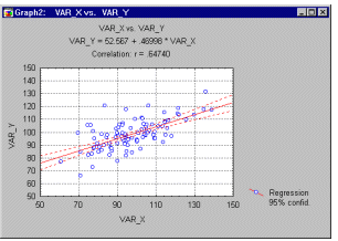
Least Squares. In the scatterplot, we have an independent or X variable, and a dependent or Y variable. These variables may, for example, represent IQ (intelligence as measured by a test) and school achievement (grade point average; GPA), respectively. Each point in the plot represents one student, that is, the respective student's IQ and GPA. The goal of linear regression procedures is to fit a line through the points. Specifically, the program will compute a line so that the squared deviations of the observed points from that line are minimized. Thus, this general procedure is sometimes also referred to as least squares estimation.
See also Exploratory Data Analysis and Data Mining Techniques, the General Stepwise Regression chapter, and the General Linear Models chapter.
The Regression Equation. A line in a two dimensional or two-variable space is defined by the equation Y=a+b*X; in full text: the Y variable can be expressed in terms of a constant (a) and a slope (b) times the X variable. The constant is also referred to as the intercept, and the slope as the regression coefficient or B coefficient. For example, GPA may best be predicted as 1+.02*IQ. Thus, knowing that a student has an IQ of 130 would lead us to predict that her GPA would be 3.6 (since, 1+.02*130=3.6).
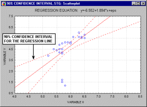
For example, the animation below shows a two dimensional regression equation plotted with three different confidence intervals (90%, 95% and 99%).
In the multivariate case, when there is more than one independent variable, the regression line cannot be visualized in the two dimensional space, but can be computed just as easily. For example, if in addition to IQ we had additional predictors of achievement (e.g., Motivation, Self- discipline) we could construct a linear equation containing all those variables. In general then, multiple regression procedures will estimate a linear equation of the form:
Y = a + b1*X1 + b2*X2 + ... + bp*Xp
Unique Prediction and Partial Correlation. Note that in this equation, the regression coefficients (or B coefficients) represent the independent contributions of each independent variable to the prediction of the dependent variable. Another way to express this fact is to say that, for example, variable X1 is correlated with the Y variable, after controlling for all other independent variables. This type of correlation is also referred to as a partial correlation (this term was first used by Yule, 1907). Perhaps the following example will clarify this issue. One would probably find a significant negative correlation between hair length and height in the population (i.e., short people have longer hair). At first this may seem odd; however, if we were to add the variable Gender into the multiple regression equation, this correlation would probably disappear. This is because women, on the average, have longer hair than men; they also are shorter on the average than men. Thus, after we remove this gender difference by entering Gender into the equation, the relationship between hair length and height disappears because hair length does not make any unique contribution to the prediction of height, above and beyond what it shares in the prediction with variable Gender. Put another way, after controlling for the variable Gender, the partial correlation between hair length and height is zero.
Predicted and Residual Scores. The regression line expresses the best prediction of the dependent variable (Y), given the independent variables (X). However, nature is rarely (if ever) perfectly predictable, and usually there is substantial variation of the observed points around the fitted regression line (as in the scatterplot shown earlier). The deviation of a particular point from the regression line (its predicted value) is called the residual value.
Residual Variance and R-square. The smaller the variability of the residual values around the regression line relative to the overall variability, the better is our prediction. For example, if there is no relationship between the X and Y variables, then the ratio of the residual variability of the Y variable to the original variance is equal to 1.0. If X and Y are perfectly related then there is no residual variance and the ratio of variance would be 0.0. In most cases, the ratio would fall somewhere between these extremes, that is, between 0.0 and 1.0. 1.0 minus this ratio is referred to as R-square or the coefficient of determination. This value is immediately interpretable in the following manner. If we have an R-square of 0.4 then we know that the variability of the Y values around the regression line is 1-0.4 times the original variance; in other words we have explained 40% of the original variability, and are left with 60% residual variability. Ideally, we would like to explain most if not all of the original variability. The R-square value is an indicator of how well the model fits the data (e.g., an R-square close to 1.0 indicates that we have accounted for almost all of the variability with the variables specified in the model).
Interpreting the Correlation Coefficient R. Customarily, the degree to which two or more predictors (independent or X variables) are related to the dependent (Y) variable is expressed in the correlation coefficient R, which is the square root of R-square. In multiple regression, R can assume values between 0 and 1. To interpret the direction of the relationship between variables, one looks at the signs (plus or minus) of the regression or B coefficients. If a B coefficient is positive, then the relationship of this variable with the dependent variable is positive (e.g., the greater the IQ the better the grade point average); if the B coefficient is negative then the relationship is negative (e.g., the lower the class size the better the average test scores). Of course, if the B coefficient is equal to 0 then there is no relationship between the variables.
| To index |
Assumptions, Limitations, Practical Considerations
Assumption of Linearity. First of all, as is evident in the name multiple linear regression, it is assumed that the relationship between variables is linear. In practice this assumption can virtually never be confirmed; fortunately, multiple regression procedures are not greatly affected by minor deviations from this assumption. However, as a rule it is prudent to always look at bivariate scatterplot of the variables of interest. If curvature in the relationships is evident, one may consider either transforming the variables, or explicitly allowing for nonlinear components.
See also Exploratory Data Analysis and Data Mining Techniques, the General Stepwise Regression chapter, and the General Linear Models chapter.
Normality Assumption. It is assumed in multiple regression that the residuals (predicted minus observed values) are distributed normally (i.e., follow the normal distribution). Again, even though most tests (specifically the F-test) are quite robust with regard to violations of this assumption, it is always a good idea, before drawing final conclusions, to review the distributions of the major variables of interest. You can produce histograms for the residuals as well as normal probability plots, in order to inspect the distribution of the residual values.
Limitations. The major conceptual limitation of all regression techniques is that one can only ascertain relationships, but never be sure about underlying causal mechanism. For example, one would find a strong positive relationship (correlation) between the damage that a fire does and the number of firemen involved in fighting the blaze. Do we conclude that the firemen cause the damage? Of course, the most likely explanation of this correlation is that the size of the fire (an external variable that we forgot to include in our study) caused the damage as well as the involvement of a certain number of firemen (i.e., the bigger the fire, the more firemen are called to fight the blaze). Even though this example is fairly obvious, in real correlation research, alternative causal explanations are often not considered.
Choice of the Number of Variables. Multiple regression is a seductive technique: "plug in" as many predictor variables as you can think of and usually at least a few of them will come out significant. This is because one is capitalizing on chance when simply including as many variables as one can think of as predictors of some other variable of interest. This problem is compounded when, in addition, the number of observations is relatively low. Intuitively, it is clear that one can hardly draw conclusions from an analysis of 100 questionnaire items based on 10 respondents. Most authors recommend that one should have at least 10 to 20 times as many observations (cases, respondents) as one has variables, otherwise the estimates of the regression line are probably very unstable and unlikely to replicate if one were to do the study over.
Multicollinearity and Matrix Ill-Conditioning. This is a common problem in many correlation analyses. Imagine that you have two predictors (X variables) of a person's height: (1) weight in pounds and (2) weight in ounces. Obviously, our two predictors are completely redundant; weight is one and the same variable, regardless of whether it is measured in pounds or ounces. Trying to decide which one of the two measures is a better predictor of height would be rather silly; however, this is exactly what one would try to do if one were to perform a multiple regression analysis with height as the dependent (Y) variable and the two measures of weight as the independent (X) variables. When there are very many variables involved, it is often not immediately apparent that this problem exists, and it may only manifest itself after several variables have already been entered into the regression equation. Nevertheless, when this problem occurs it means that at least one of the predictor variables is (practically) completely redundant with other predictors. There are many statistical indicators of this type of redundancy (tolerances, semi-partial R, etc., as well as some remedies (e.g., Ridge regression).
Fitting Centered Polynomial Models. The fitting of higher-order polynomials of an independent variable with a mean not equal to zero can create difficult multicollinearity problems. Specifically, the polynomials will be highly correlated due to the mean of the primary independent variable. With large numbers (e.g., Julian dates), this problem is very serious, and if proper protections are not put in place, can cause wrong results! The solution is to "center" the independent variable (sometimes, this procedures is referred to as "centered polynomials"), i.e., to subtract the mean, and then to compute the polynomials. See, for example, the classic text by Neter, Wasserman, & Kutner (1985, Chapter 9), for a detailed discussion of this issue (and analyses with polynomial models in general).
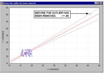
The Importance of Residual Analysis. Even though most assumptions of multiple regression cannot be tested explicitly, gross violations can be detected and should be dealt with appropriately. In particular outliers (i.e., extreme cases) can seriously bias the results by "pulling" or "pushing" the regression line in a particular direction (see the animation below), thereby leading to biased regression coefficients. Often, excluding just a single extreme case can yield a completely different set of results.
| To index |
