Uniform Distribution. The discrete Uniform distribution (the term first used by Uspensky, 1937) has density function:

f(x) = 1/N          x = 1, 2, ..., N

The continuous Uniform distribution has density function: where

f(x) = 1/(b-a)        a < x < b

a     is the lower limit of the interval from which points will be selected
b     is the upper limit of the interval from which points will be selected

Unimodal Distribution. A distribution that has only one mode. A typical example is the normal distribution which happens to be also symmetrical but many unimodal distributions are not symmetrical (e.g., typically the distribution of income is not symmetrical but "left-skewed"; see skewness). See also bimodal distribution, multimodal distribution.

Unit Penalty. In several search algorithms, a penalty factor which is multiplied by the number of units in the network and added to the error of the network, when comparing the performance of the network with others. This has the effect of selecting smaller networks at the expense of larger ones. See also, Penalty Function.

Unit Types (in Neural Networks). Units in the input layer are extremely simple: they simply hold an output value, which they pass onto units in the second layer. Input units do no processing. Input units have their synaptic function set to Dot Product, and their activation function set to Identity by default; actually these functions are ignored in input units.

Each hidden or output unit has a number of incoming connections from units in the preceding layer (the fan-in): one for each unit in the preceding layer. Each unit also has a threshold value.

The outputs of the units in the preceding layer, the weights on the associated connections, and the threshold value are fed through the unit's synaptic function (post synaptic potential function) to produce a single value (the unit's input value).

The input value is passed through the unit's activation function to produce a single output value, also known as the activation level of the unit.

Unsupervised learning algorithms require a data set that includes typical input variable values. Observed output variable values are not required. If output variable values are present in the data set, they are simply ignored.

Center Assignment

Kohonen Algorithm

Radial Sampling

K-Means Algorithm

Deviation Assignment

Explicit Deviation Assignment

Isotropic Deviation Assignment

K-Nearest Neighbor

Principal Components Analysis

Principal Components Analysis

Variance. The variance (this term was first used by Fisher, 1918a) of a population of values is computed as:

² = (x_i-µ)²/N

where
µ    is the population mean
N   is the population size.
The unbiased sample estimate of the population variance is computed as:

s² = (x_i-xbar)²/n-1

where
xbar   is the sample mean
n        is the sample size.

See also, Descriptive Statistics.

Variance Components (in Mixed Model ANOVA) The term variance components is used in the context of experimental designs with random effects, to denote the estimate of the (amount of) variance that can be attributed to those effects. For example, if one were interested in the effect that the quality of different schools has on academic proficiency, one could select a sample of schools to estimate the amount of variance in academic proficiency (component of variance) that is attributable to differences between schools.

See also, Analysis of Variance and Variance Components and Mixed Model ANOVA/ANCOVA.

Variance Inflation Factor (VIF). The diagonal elements of the inverse correlation matrix (i.e., -1 times the diagonal elements of the sweep matrix) for variables that are in the equation are also sometimes called variance inflation factors (VIF; e.g., see Neter, Wasserman, Kutner, 1985). This terminology denotes the fact that the variances of the standardized regression coefficients can be computed as the product of the residual variance (for the correlation transformed model) times the respective diagonal elements of the inverse correlation matrix. If the predictor variables are uncorrelated, then the diagonal elements of the inverse correlation matrix are equal to 1.0; thus, for correlated predictors, these elements represent an "inflation factor" for the variance of the regression coefficients, due to the redundancy of the predictors.

See also, Multiple Regression.

V-fold Cross-validation. In v-fold cross-validation, repeated (v) random samples are drawn from the data for the analysis, and the respective model or prediction method, etc. is then applied to compute predicted values, classifications, etc. Typically, summary indices of the accuracy of the prediction are computed over the v replications; thus, this technique allows the analyst to evaluate the overall accuracy of the respective prediction model or method in repeatedly drawn random samples. This method is customarily used in tree classification and regression.

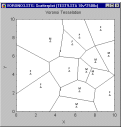
Voronoi. The Voronoi tessellation graph plots values of two variables X and Y in a scatterplot, then divides the space between individual data points into regions such that the boundaries surrounding each data point enclose an area that is closer to that data point than to any other neighboring points.

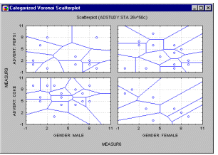
Voronoi Scatterplot. This specialized univariate scatterplot is more an analytic technique than just a method to graphically present data. The solutions it offers, help to model a variety of phenomena in natural and social sciences (e.g., Coombs, 1964; Ripley, 1981). The program divides the space between the individual data points represented by XY coordinates in 2D space. The division is such that each of the data points is surrounded by boundaries including only the area that is closer to its respective "center" data point than to any other data point.

The particular ways in which this method is used depends largely on specific research areas, however, in many of them, it is helpful to add additional dimensions to this plot by using categorization options (as shown in the example below).

See also, Data Reduction.

Voting. See Bagging.

W = * 1/Var() *

In this formula, stands for the parameter estimates, and Var() stands for the asymptotic variance of the parameter estimates. The Wald statistic is tested against the Chi-square distribution.

WebSTATISTICA Server applications. Web STATISTICA Server is the ultimate enterprise system that offers the full Web enablement, including the ability to run STATISTICA interactively or in batch from a Web browser on any computer (incl. Linux, UNIX), offload time consuming tasks to the servers (using distributed processing), use multi-tier client/server architecture, manage projects over the Web, and collaborate "across the hall or across continents."

It enables users to:
Work collaboratively "across the hall" or "across continents"
Run STATISTICA using any computer in the world (connected to the Internet)
Offload time consuming tasks to the servers
Manage/administer projects over the Web
Develop highly customized Web applications
and much, much more…


Weibull Distribution. The Weibull distribution (Weibull, 1939, 1951; see also Lieblein, 1955) has density function (for positive parameters b, c, and ):

f(x) = c/b*[(x-)/b]^c-1 * e^{-[(x-)/b]^c}
< x,  b > 0,  c > 0

where
b     is the scale parameter of the distribution
c     is the shape parameter of the distribution
   is the location parameter of the distribution
e     is the base of the natural logarithm, sometimes called Euler's e (2.71...)

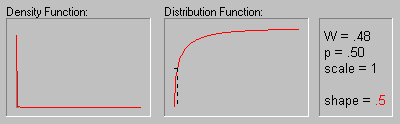
The animation above shows the Weibull distribution as the shape parameter increases (.5, 1, 2, 3, 4, 5, and 10).

Weigend Weight Regularization (in Neural Networks).

A common problem in neural network training (particularly of multilayer perceptrons) is over-fitting. A network with a large number of weights in comparison with the number of training cases available can achieve a low training error by modeling a function that fits the training data well despite failing to capture the underlying model. An over-fitted model typically has high curvature, as the function is contorted to pass through the points, modeling any noise in addition to the underlying data.

There are several approaches in neural network training to deal with the over-fitting problem (Bishop, 1995). These approaches are listed below.

• Select a neural network with just enough units to model the underlying function. The problem with this approach is determining the correct number of units, which is problem-dependent.

• Add some noise to the training cases during training (altering the noise on each case each epoch): this "blurs" the position of the training data, and forces the network to model a smoothed version of the data.

• Stop training (see Stopping Conditions) when the selection error begins to rise, even if the training error continues to fall. This event is a sure sign that the network is beginning to over-fit the data.

• Use a regularization technique, which explicitly penalizes networks with large curvature, thus encouraging the development of a smoother model.

The last technique mentioned is regularization, and this section describes Weigend weight regularization (Weigend et. al., 1991).

A multilayer perceptron model with sigmoid (logistic or hyperbolic tangent) activation functions has higher curvature if the weights are larger. You can see this by considering the shape of the sigmoid curve: if you just look at a small part of the central section, around the value 0.0, it is "nearly linear," and so a network with very small weights will model a "nearly linear" function, which has low curvature. As an aside, note that during training the weights are first set to small values (corresponding to a low curvature function), and then (at least some of them) diverge. One way to promote low curvature therefore is to encourage smaller weights.

Weigend weight regularization does this by adding an extra term to the error function, which penalizes larger weights. Hence the network tends to develop the larger weights that it needs to model the problem, and the others are driven toward zero. The technique can be used with any multilayer perceptron training algorithms (back propagation, conjugate gradient descent, Quasi-Newton Method, quick propagation, and Delta-bar-Delta) apart from Levenberg-Marquardt, which makes its own assumptions about the error function.

The technique is commonly referred to as Weigend weight elimination, as it is possible, once weights become very small, to simply remove them from the network. This is an extremely useful technique for developing models with a "sensible" number of hidden units, and for selecting input variables.

Once a model has been trained with Weigend regularization and excess inputs and hidden units removed, it can be further trained with Weigend regularization turned off, to "sharpen up" the final solution.

Weigend regularization can also be very helpful in that it tends to prevent models from becoming over-fitted.

Note: When using Weigend regularization, the error on the progress graph includes the Weigend penalty factor. If you compare a network trained with Weigend to one without, you may get a false impression that the Weigend-trained network is under-performing. To compare such networks, view the error reported in the summary statistics on the model list (this does not include the Weigend error term).

Technical Details. The Weigend error penalty is given by:

where l is the Regularization coefficient, wi is each of the weights, and wo is the Scale coefficient.

The error penalty is added to the error calculated by the network's error function during training, and its derivative is added to the weight's derivative. However, the penalty is ignored when running a network.

The regularization coefficient is usually manipulated to adjust the selective pressure to prune units. The relationship between this coefficient and the number of active units is roughly logarithmic, so the coefficient is typically altered over a wide range (0.01-0.0001, say).

The scale coefficient defines what is a "large" value to the algorithm. The default setting of 1.0 is usually reasonable, and it is seldom altered.

A feature of the Weigend error penalty is that it does not just penalize larger weights. It also prefers to tolerate an uneven mix of some large and some small weights, as opposed to a number of medium-sized weights. It is this property that allows it to "eliminate" weights.

Wilcoxon test. The Wilcoxon test is a nonparametric alternative to t-test for dependent samples. It is designed to test a hypothesis about the location (median) of a population distribution. It often involves the use of matched pairs, for example, "before" and "after" data, in which case it tests for a median difference of zero.

This procedure assumes that the variables under consideration were measured on a scale that allows the rank ordering of observations based on each variable (i.e., ordinal scale) and that allows rank ordering of the differences between variables (this type of scale is sometimes referred to as an ordered metric scale, see Coombs, 1950). For more details, see Siegel & Castellan, 1988. See also, Nonparametric Statistics.

Win Frequencies (in Neural Networks). In a Kohonen network, the number of times that each radial unit is the winner when the data set is executed. Units which win frequently represent cluster centers in the topological map. See, Neural Networks.

Wire. A wire is a line, usually curved, used in a path diagram to represent variances and covariances of exogenous variables.