In addition, for sigma restricted models (e.g., in General Regression Models; some software offers the user a choice between the sigma restricted and overparameterized models), we propose a Type VI sums of squares option; this approach is identical to what is described as the effective hypothesis method in Hocking (1996). For details regarding these methods, refer to the Six types of sums of squares topic of the General Linear Model chapter.

Efficient score statistic. See Score statistic.

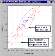
Ellipse, Prediction Interval (Area) and Range.
Prediction Interval (Area) Ellipse: This type of ellipse is useful for establishing confidence intervals for the prediction of single new observations (prediction intervals). Such bivariate confidence or control limits are, for example, often used in the context of multivariate control charts for industrial quality control (see, for example, Montgomery, 1996; see also Hotelling T-square chart).

The ellipse is determined based on the assumption that the two variables follow the bivariate normal distribution. The orientation of this ellipse is determined by the sign of the linear correlation between two variables (the longer axis of the ellipse is superimposed on the regression line). The probability that the values will fall within the area marked by the ellipse is determined by the value of the coefficient that defines the ellipse (e.g., 95%). For additional information see, for example, Tracy, Young, and Mason (1992), or Montgomery 1996); see also the description of the prediction interval ellipse.
Range Ellipse: This type of ellipse is a fixed size ellipse determined such that the length of its horizontal and vertical projection onto the X- and Y-axis (respectively) is equal to the mean (Range * I) where the mean and range refer to the X or Y variable, and I is the current value of the coefficient field.

Endogenous Variable. An endogenous variable is a variable that appears as a dependent variable in at least one equation in a structural model. In a path diagram, endogenous variables can be recognized by the fact that they have at least one arrow pointing to them.

Ensembles (in Neural Networks). Ensembles are collections of neural networks that cooperate in performing a prediction.

Output ensembles. Output ensembles are the most general form. Any combination of networks can be combined in an output ensemble. If the networks have different outputs, the resulting ensemble simply has multiple outputs. Thus, an output ensemble can be used to form a multiple output model where each output's prediction is formed separately.

If any networks in the ensemble have a shared output, the ensemble estimates a value for that output by combining the outputs from the individual networks. For classification (nominal outputs), the networks' predictions are combined in a winner-takes-all vote - the most common class among the combined networks is used. In the event of a tie, the "unknown" class is returned. For regression (numeric variables), the networks' predictions are averaged. In both cases, the vote or average is weighted using the networks' membership weights in the ensemble (usually all equal to 1.0).

Confidence ensembles. Confidence ensembles are much more restrictive than output ensembles. The network predictions are combined at the level of the output neurons. To make sense, the encoding of the output variables must therefore be the same for all the members. Given that restriction, there is no point in forming confidence ensembles for regression problems, as the effect is to produce the same output as an output ensemble, but with the averaging performed before scaling rather than after. Confidence ensembles are designed for use with classification problems.

The advantage of using a confidence ensemble for a classification problem is that it can estimate overall confidence levels for the various classes, rather than simply providing a final choice of class.

Why use ensembles?

There are a number of uses for ensembles:

• Ensembles can conveniently group together networks that provide predictions for related variables without requiring that all those variables be combined into a single network. Multiple output networks often suffer from cross-talk in the hidden neurons, and make ineffective predictions. Using an ensemble, each output can be predicted separately.

• Ensembles provide an important method to combat over-learning and improve generalization. Averaging predictions across models with different structures, and/or trained on different data subsets, can reduce model variance without increasing model bias. This is a relatively simple way to improve generalization. Ensembles therefore are particularly effective when combined with resampling. An important piece of theory shows that the expected performance of an ensemble is greater than or equal to the average performance of the members.

• Ensembles report the average performance and error measures of their member networks. You can perform resampling experiments, and save the results to an ensemble. Then, these average measures give an unbiased estimate of an individual network's performance, if trained in the same fashion. It is standard practice to use resampling techniques such as cross validation to estimate network performance in this fashion.

See also, Enterprise-wide Software Systems.

Enterprise SPC. Enterprise SPC is a groupware based process control system (see SPC), designed to work in enterprise-wide environment and allowing engineers and supervisors to share data, chart specifications (and other QC criteria), reports, and database queries. Enterprise SPC systems always include central QC data bases and if properly integrated, they allow the managers to maintain quality standards for all products/processes in a given corporation.

See also, Statistical Process Control, Quality Control, Process Analysis and STATISTICA Enterprise-wide SPC System (SEWSS).

For more information on process control systems, see the ASQC/AIAG's Fundamental statistical process control reference manual (1991).

Enterprise-Wide Software Systems. Software applications designed to work in enterprise computer envirnoments (e.g., such as large corporate computer systems). Such applications typically feature extensive groupware functionality, and they are usually well integrated with large repositories of data stored in corporate data warehouses. See also Data Warehousing.

Epoch (in Neural Networks). During iterative training of a neural network, an Epoch is a single pass through the entire training set, followed by testing of the verification set.

For more information, see the Neural Networks chapter.

Error Bars (2D Box Plots). In this style of 2D Box plots, the ranges or error bars are calculated from the data. The central tendency (e.g., median or mean), and range or variation statistics (e.g., min-max values, quartiles, standard errors, or standard deviations) are computed for each variable and the selected values are presented as error bars.

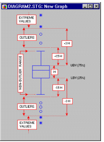
The diagram above illustrates the ranges of outliers and extremes in the "classic" box and whisker plot (for more information about box plots, see Tukey, 1977).

Error Bars (2D Range Plots). In this style of 2D Range Plot, the ranges or error bars are defined by the raw values in the selected variables. The midpoints are represented by point markers. One range or error bar is plotted for each case. In the simplest instance, three variables need to be selected, one representing the mid-points, one representing the upper limits and one representing the lower limits.

Error Bars (3D Box Plots). In this style of 3D Sequential Box Plot, the ranges of values of selected variables are plotted separately for groups of cases defined by values of a categorical (grouping) variable. The central tendency (e.g., median or mean), and range or variation statistics (e.g., min-max values, quartiles, standard errors, or standard deviations) are computed for each variable and for each group of cases and the selected values are presented as error bars.

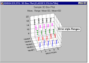
3D Range plots differ from 3D Box plots in that for Range plots, the ranges are the values of the selected variables (e.g., one variable contains the minimum range values and another variable contains the maximum range values) while for Box plots the ranges are calculated from variable values (e.g., standard deviations, standard errors, or min-max value).

Error Bars (3D Range Plots). In this style of 3D Sequential Range Plot, the error bars are not calculated from data but defined by the raw values in the selected variables. The midpoints are represented by point markers. One error bar is plotted for each case. The range variables can be interpreted either as absolute values or values representing deviations from the midpoint depending on the current setting of the Mode option in the graph definition dialog. Single or multiple variables can be represented in the graph.

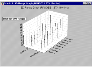
3D Range plots differ from 3D Box plots in that for Range plots, the ranges are the values of the selected variables (e.g., one variable contains the minimum range values and another variable contains the maximum range values) while for Box plots, the ranges are calculated from variable values (e.g., standard deviations, standard errors, or min-max values).

Error Function (in Neural Networks). The error function is used in training the network and in reporting the error. The error function used can have a profound effect on the performance of training algorithms (Bishop, 1995).

The following four error functions are available.

Sum-squared. The error is the sum of the squared differences between the target and actual output values on each output unit. This is the standard error function used in regression problems. It can also be used for classification problems, giving robust performance in estimating discriminant functions, although arguably entropy functions are more appropriate for classification, as they correspond to maximum likelihood decision making (on the assumption that the generating distribution is drawn from the exponential family), and allow outputs to be interpreted as probabilities.

City-block. The error is the sum of the differences between the target and actual output values on each output unit; differences are always taken to be positive. The city-block error function is less sensitive to outlying points than the sum-squared error function (where a disproportionate amount of the error can be accounted for by the worst-behaved cases). Consequently, networks trained with this metric may perform better on regression problems if there are a few wide-flung outliers (either because the data naturally has such a structure, or because some cases may be mislabeled).

Cross-entropy (single & multiple). This error is the sum of the products of the target value and the logarithm of the error value on each output unit. There are two versions: one for single-output (two-class) networks, the other for multiple-output networks. The cross-entropy error function is specially designed for classification problems, where it is used in combination with the logistic (single output) or softmax (multiple output) activation functions in the output layer of the network. This is equivalent to maximum likelihood estimation of the network weights. An MLP with no hidden layers, a single output unit, and cross entropy error function is equivalent to a standard logistic regression function (logit or probit classification).

Kohonen. The Kohonen error assumes that the second layer of the network consists of radial units representing cluster centers. The error is the distance from the input case to the nearest of these. The Kohonen error function is intended for use with Kohonen networks and Cluster networks only.

f=Lb

where L is a vector of coefficients, will also in general not be unique. However, Lb for an L which satisfies

L=L(X'X)`X'X

is invariant for all possible generalized inverses, and is therefore called an estimable function.

See also general linear model, generalized linear model, design matrix, matrix rank, generalized inverse; for additional details, see also General Linear Models.

Euclidean Distance. One can think of the independent variables (in a regression equation) as defining a multidimensional space in which each observation can be plotted. The Euclidean distance is the geometric distance in that multidimensional space. It is computed as:

distance(x,y)={S_i (x_i - y_i )²}^1/2

Note that Euclidean (and squared Euclidean) distances are computed from raw data, and not from standardized data. For more information on Euclidean distances and other distance measures, see Distance Measures in the Cluster Analysis chapter.

Euler's e. The base of the natural logarithm (numerical value: 2.71828182834905...), named after the Swiss mathematician Leonhard Euler (1707-1783).

Exogenous Variable. An exogenous variable is a variable that never appears as a dependent variable in any equation in a structural model. In a path diagram, exogenous variables can be recognized by the fact that they have no arrows pointing to them.

Experimental Design (DOE, Industrial Experimental Design). In industrial settings, Experimental design (DOE) techniques apply analysis of variance principles to product development. The primary goal is usually to extract the maximum amount of unbiased information regarding the factors affecting a production process from as few (costly) observations as possible. In industrial settings, complex interactions among many factors that influence a product are often regarded as a "nuisance" (they are often of no interest; they only complicate the process of identifying important factors, and in experiments with many factors it would not be possible or practical to identify them anyway). Hence, if you review standard texts on experimentation in industry (Box, Hunter, and Hunter, 1978; Box and Draper, 1987; Mason, Gunst, and Hess, 1989; Taguchi, 1987) you will find that they will primarily discuss designs with many factors (e.g., 16 or 32) in which interaction effects cannot be evaluated, and the primary focus of the discussion is how to derive unbiased main effect (and, perhaps, two-way interaction) estimates with a minimum number of observations.

For more information, see the Experimental Design chapter.

Explained variance. The proportion of the variability in the data which is accounted for by the model (e.g., in Multiple Regression, ANOVA, Nonlinear Estimation, Neural Networks) .

Exploratory Data Analysis (EDA). As opposed to traditional hypothesis testing designed to verify a priori hypotheses about relations between variables (e.g., "There is a positive correlation between the AGE of a person and his/her RISK TAKING disposition"), exploratory data analysis (EDA) is used to identify systematic relations between variables when there are no (or not complete) a priori expectations as to the nature of those relations. In a typical exploratory data analysis process, many variables are taken into account and compared, using a variety of techniques in the search for systematic patterns.

For more information, see Exploratory Data Analysis (EDA) and Data Mining Techniques.

Exponential Function. This fits to the data, an exponential function of the form:

y = b*exp(q*x)

Exponential Distribution. The exponential distribution function is defined as:

f(x) = * e^-x
0 x < , > 0

where
   (lambda) is an exponential function parameter (an alternative parameterization is scale parameter b=1/)
 e      is the base of the natural logarithm, sometimes called Euler's e (2.71...)

The graphic above shows the shape of the Exponential distribution when lambda equals 1.

Exponential Family of Distributions.

A family of probability distributions with exponential terms, which includes many of the most important distributions encountered in real (neural network) problems (including the normal, or Gaussian distribution, and the alpha and beta distributions). See also, Neural Networks.

Exponentially Weighted Moving Average Line. This type of moving average can be considered to be a generalization of the simple moving average. Specifically, we could compute each data point for the plot as:

z_t = *x-bar_t + (1-)*z _t-1

In this formula, each point z_t is computed as (lambda) times the respective mean x- bar_t, plus one minus times the previous (computed) point in the plot. The parameter (lambda) here should assume values greater than 0 and less than 1. You may recognize this formula as the common exponential smoothing formula. Without going into detail (see Montgomery, 1985, p. 239), this method of averaging specifies that the weight for historically "old" sample means decreases geometrically as one continues to draw samples. This type of moving average line also smoothes the pattern of means across samples, and allows the engineer to detect trends more easily.

Extrapolation. Predicting the value of unknown data points by projecting a function beyond the range of known data points.

Extreme Values (in Box Plots). Values which are "far" from the middle of the distribution are referred to as outliers and extreme values if they meet certain conditions.

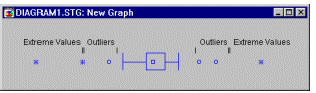
A data point is deemed to be an extreme value if the following conditions hold:

data point value > UBV + 2*o.c.*(UBV - LBV)
or
data point value < LBV - 2*o.c.*(UBV - LBV)

where
UBV    is the upper value of the box in the box plot (e.g., the mean + standard error or the 75th percentile).
LBV    is the lower value of the box in the box plot (e.g., the mean - standard error or the 25th percentile).
o.c.      is the outlier coefficient (when this coefficient equals 1.5, the extreme values are those which are outside the 3 box length range from the upper and lower value of the box).

For example, the following diagram illustrates the ranges of outliers and extremes in the "classic" box and whisker plot (for more information about box plots, see Tukey, 1977).

Extreme Value Distribution. The extreme value (Type I) distribution (the term first used by Lieblein, 1953) has the probability density function:

f(x) = 1/b * e^-(x-a)/b * e^{-e-(x-a) / b}
- < x <
b > 0

where
a    is the location parameter
b    is the scale parameter
e    is the base of the natural logarithm, sometimes called Euler's e (2.71...)
This distribution is also sometimes referred to as the distribution of the largest extreme.

See also, Process Analysis.

The graphic above shows the shape of the extreme value distribution when the location parameter equals 0 and the scale parameter equals 1.