Quality. The term Quality in the context of correspondence analysis pertains to the quality of representation of the respective row point in the coordinate system defined by the respective numbers of dimensions, as chosen by the user. The quality of a point is defined as the ratio of the squared distance of the point from the origin in the chosen number of dimensions, over the squared distance from the origin in the space defined by the maximum number of dimensions (remember that the metric in the typical correspondence analysis is Chi-square). By analogy to Factor Analysis, the quality of a point is similar in its interpretation to the communality for a variable in factor analysis.

A low quality means that the current number of dimensions does not represent well the respective row (or column).

Quality Control. In all production processes, the extent to which products meet quality specifications must be monitored. In the most general terms, there are two "enemies" of product quality: (1) deviations from target specifications, and (2) excessive variability around target specifications. During the earlier stages of developing the production process, designed experiments are often used to optimize these two quality characteristics (see Experimental Design); the methods discussed in the Quality Control chapter are on-line or in-process quality control procedures to monitor an on-going production process.

The general approach to on-line quality control is straightforward: We simply extract samples of a certain size from the ongoing production process. We then produce line charts of the variability in those samples, and consider their closeness to target specifications. If a trend emerges in those lines, or if samples fall outside pre-specified limits, then we declare the process to be out of control and take action to find the cause of the problem. These types of charts are sometimes also referred to as Shewhart control charts (named after W. A. Shewhart who is generally credited as being the first to introduce these methods; see Shewhart, 1931).

For more information, see the Quality Control Charts chapter.

Quantiles. The quantile (this term was first used by Kendall, 1940) of a distribution of values is a number x_p such that a proportion p of the population values are less than or equal to x_p. For example, the .25 quantile (also referred to as the 25th percentile or lower quartile) of a variable is a value (x_p) such that 25% (p) of the values of the variable fall below that value.

Similarly, the .75 quantile (also referred to as the 75th percentile or upper quartile) is a value such that 75% of the values of the variable fall below that value and is calculated accordingly.

See also, Quantile-Quantile Plots

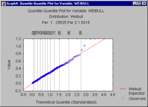
Quantile-Quantile Plots. You can visually check for the fit of a theoretical distribution to the observed data by examining the quantile-quantile (or Q-Q) plot (also called Quantile Plot).

In this plot, the observed values of a variable are plotted against the theoretical quantiles. A good fit of the theoretical distribution to the observed values would be indicated by this plot if the plotted values fall onto a straight line. To produce a Q-Q plot, the program will first sort the n observed data points into ascending order, so that:

x₁ x₂ ... x_n

These observed values are plotted against one axis of the graph; on the other axis the plot will show:

F^-1((i-r_adj) / (n+n_adj))

where i is the rank of the respective observation, r_adj and n_adj are adjustment factors (0.5) and F^-1 denotes the inverse of the probability integral for the respective standardized distribution. The resulting plot (see below) is a scatterplot of the observed values against the (standardized) expected values, given the respective distribution. Note also that the adjustment factors r_adj and n_adj ensure that the p-value for the inverse probability integral will fall between 0 and 1, but not including 0 and 1 (see Chambers, Cleveland, Kleiner, and Tukey, 1983.

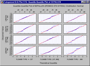
Quantile-Quantile Plots - Categorized. In this graph, you can visually check for the fit of a theoretical distribution to the observed data by examining each quantile-quantile (or Q-Q) plot (also called Quantile Plot, see Quantile-Quantile Plots) for the respective level of the grouping variable (or user-defined subset of data).

In this plot, the observed values of a variable are plotted against the theoretical quantiles. A good fit of the theoretical distribution to the observed values would be indicated by this plot if the plotted values fall onto a straight line. One component graph is produced for each level of the grouping variable(or user-defined subset of data) and all the component graphs are arranged in one display to allow for comparisons between the subsets of data (categories). (See Quantile-Quantile Plots for more details on how to produce a Q-Q plot.)

Quartile Range. The quartile (this term was first used by Galton, 1882) range of a variable is calculated as the value of the 75th percentile minus the value of the 25th percentile. Thus it is the width of the range about the median that includes 50% of the cases.

For more information, see Nonparametrics

Quartiles. The lower and upper quartiles (this term was first used by Galton, 1882; also referred to as the .25 and .75 quantiles) are the 25th and 75th percentiles of the distribution (respectively). The 25th percentile of a variable is a value such that 25% of the values of the variable fall below that value.

Similarly, the 75th percentile is a value such that 75% of the values of the variable fall below that value and is calculated accordingly.

Quasi-Newton Method (in Neural Networks). Quasi-Newton (Bishop, 1995; Shepherd, 1997) is an advanced method of training multilayer perceptrons. It usually performs significantly better than Back Propagation, and can be used wherever back propagation can be. It is the recommended technique for most networks with a small number of weights (less than a couple of hundred). If the network is a single output regression network and the problem has low residuals, then Levenberg-Marquardt may perform better.

Quasi-Newton is a batch update algorithm: whereas back propagation adjusts the network weights after each case, Quasi-Newton works out the average gradient of the error surface across all cases before updating the weights once at the end of the epoch.

For this reason, there is no shuffle option available with Quasi-Newton, since it would clearly serve no useful function. There is also no need to select learning or momentum rates for Quasi-Newton, so it can be much easier to use than back propagation. Additive noise would destroy the assumptions made by Quasi-Newton about the shape of search space, and so is also not available.

Quasi-Newton works by exploiting the observation that, on a quadratic (i.e. parabolic) error surface, one can step directly to the minimum using the Newton step - a calculation involving the Hessian matrix (the matrix of second partial derivatives of the error surface). Any error surface is approximately quadratic "close to" a minimum. Since, unfortunately, the Hessian matrix is difficult and expensive to calculate, and anyway the Newton step is likely to be wrong on a non-quadratic surface, Quasi-Newton iteratively builds up an approximation to the inverse Hessian. The approximation at first follows the line of steepest descent, and later follows the estimated Hessian more closely.

Quasi-Newton is the most popular algorithm in nonlinear optimization, with a reputation for fast convergence. It does, however, has some drawbacks - it is rather less numerically stable than, say, Conjugate Gradient Descent, it may be inclined to converge to local minima, and the memory requirements are proportional to the square of the number of weights in the network.

It is often beneficial to precede Quasi-Newton training with a short burst of Back Propagation (say 100 epochs), to cut down on problems with local minima.

If the network has many weights, you are advised to use Conjugate Gradient Descent instead. Conjugate Gradient Descent has memory requirements proportional only to the number of weights, not the square of the number of weights, and the training time is usually comparable with Quasi-Newton, if somewhat slower.

Technical Details. Quasi-Newton is batch-based; it calculates the error gradient as the sum of the error gradients on each training case.

It maintains an approximation to the inverse Hessian matrix, called H below. The direction of steepest descent is called g below. The weight vector on the ith epoch is referred to as fi below. H is initialized to the identity matrix, so that the first step is in the direction g (i.e. the same direction as that chosen by Back Propagation). On each epoch, a back tracking line search is performed in the direction:

d = – Hg

Subsequently, the search direction is updated using the BFGS (Broyden-Fletcher-Goldfarb-Shanno) formula:

This is "guaranteed" to maintain a positive-definite approximation (i.e. it will always indicate a descent direction), and to converge to the true inverse Hessian in W steps, where W is the number of weights, on a quadratic error surface.  In practice, numerical errors may violate these theoretical guarantees and lead to divergence of weights or other modes of failure. In this case, run the algorithm again, or choose a different training algorithm.

Quick Propagation (in Neural Networks). Despite the name, quick propagation (Fahlman, 1988; Patterson, 1996) is not necessarily faster than back propagation, although it may prove significantly faster for some applications.

Quick propagation also sometimes seems more inclined to instability and to getting stuck in local minima, than back propagation; these tendencies may determine whether quick propagation is more appropriate for a particular problem.

Quick propagation is a batch update algorithm: whereas back propagation adjusts the network weights after each case, quick propagation works out the average gradient of the error surface across all cases before updating the weights once at the end of the epoch.

For this reason, there is no shuffle option available with quick propagation, since it would clearly serve no useful function.

Quick propagation works by making the (typically ill-founded) assumption that the error surface is locally quadratic, with the axes of the hyper-ellipsoid error surface aligned with the weights. If this is true, then the minimum of the error surface can be found after only a couple of epochs. Of course, the assumption is not generally valid, but if it is even close to true, the algorithm can converge on the minimum very rapidly.

Based on this assumption, quick propagation works as follows:

On the first epoch, the weights are adjusted using the same rule as back propagation, based upon the local gradient and the learning rate.

On subsequent epochs, the quadratic assumption is used to attempt to move directly to the minimum.

The basic quick propagation formula suffers from a number of numerical problems. First, if the error surface is not concave, the algorithm can actually go the wrong way. If the gradient changes little or not at all, the change can be extremely large, or even infinite! Finally, if a zero gradient is encountered, a weight will stop changing permanently.

Technical Details. Quick propagation is batch-based; it calculates the error gradient as the sum of the error gradients on each training case.

On the first epoch, quick propagation updates weights just like back propagation.

Subsequently, weight changes are calculated using the quick propagation formula:

This formula is numerically unstable if s(t) is very close to, equal to, or greater than s(t-1). Since s(t) is discovered after a move along the direction of the gradient, such conditions can only occur if the slope becomes constant, or becomes steeper (i.e., it is not concave).

In these cases, the weight update formula is:

a - the acceleration coefficient.

If the gradient becomes zero, then the weight delta becomes zero, and by the above formulae remains zero permanently even if the gradient subsequently changes. A conventional approach to solve this problem is to add a small factor to the weight changes calculated above. However, this approach can cause numerical instability.

See also, Neural Networks.