For additional information about generalized linear models, see also Dobson (1990), Green and Silverman (1994), or McCullagh and Nelder (1989).
The Generalized Linear Model (GLZ) is a generalization of the general linear model (see, e.g., the General Linear Models, Multiple Regression, and ANOVA/MANOVA chapters). In its simplest form, a linear model specifies the (linear) relationship between a dependent (or response) variable Y, and a set of predictor variables, the X's, so that
Y = b0 + b1X1 + b2X2 + ... + bkXk
In this equation b0 is the regression coefficient for the intercept and the bi values are the regression coefficients (for variables 1 through k) computed from the data.
So for example, one could estimate (i.e., predict) a person's weight as a function of the person's height and gender. You could use linear regression to estimate the respective regression coefficients from a sample of data, measuring height, weight, and observing the subjects' gender. For many data analysis problems, estimates of the linear relationships between variables are adequate to describe the observed data, and to make reasonable predictions for new observations (see the Multiple Regression chapter for additional details).
However, there are many relationships that cannot adequately be summarized by a simple linear equation, for two major reasons:
Distribution of dependent variable. First, the dependent variable of interest may have a non-continuous distribution, and thus, the predicted values should also follow the respective distribution; any other predicted values are not logically possible. For example, a researcher may be interested in predicting one of three possible discrete outcomes (e.g., a consumer's choice of one of three alternative products). In that case, the dependent variable can only take on 3 distinct values, and the distribution of the dependent variable is said to be multinomial. Or suppose you are trying to predict people's family planing choices, specifically, how many children families will have, as a function of income and various other socioeconomic indicators. The dependent variable -- number of children -- is discrete (i.e., a family may have 1, 2, or 3 children and so on, but cannot have 2.4 children), and most likely the distribution of that variable is highly skewed (i.e., most families have 1, 2, or 3 children, fewer will have 4 or 5, very few will have 6 or 7, and so on). In this case it would be reasonable to assume that the dependent variable follows a Poisson distribution.
Link function. A second reason why the linear (multiple regression) model might be inadequate to describe a particular relationship is that the effect of the predictors on the dependent variable may not be linear in nature. For example, the relationship between a person's age and various indicators of health is most likely not linear in nature: During early adulthood, the (average) health status of people who are 30 years old as compared to the (average) health status of people who are 40 years old is not markedly different. However, the difference in health status of 60 year old people and 70 year old people is probably greater. Thus, the relationship between age and health status is likely non-linear in nature. Probably some kind of a power function would be adequate to describe the relationship between a person's age and health, so that each increment in years of age at older ages will have greater impact on health status, as compared to each increment in years of age during early adulthood. Put in other words, the link between age and health status is best described as non-linear, or as a power relationship in this particular example.
The generalized linear model can be used to predict responses both for dependent variables with discrete distributions and for dependent variables which are nonlinearly related to the predictors.
| To index |
To summarize the basic ideas, the generalized linear model differs from the general linear model (of which, for example, multiple regression is a special case) in two major respects: First, the distribution of the dependent or response variable can be (explicitly) non-normal, and does not have to be continuous, i.e., it can be binomial, multinomial, or ordinal multinomial (i.e., contain information on ranks only); second, the dependent variable values are predicted from a linear combination of predictor variables, which are "connected" to the dependent variable via a link function. The general linear model for a single dependent variable can be considered a special case of the generalized linear model: In the general linear model the dependent variable values are expected to follow the normal distribution, and the link function is a simple identity function (i.e., the linear combination of values for the predictor variables is not transformed).
To illustrate, in the general linear model a response variable Y is linearly associated with values on the X variables by
Y = b0 + b1X1 + b2X2 + ... + bkXk) + e
(where e stands for the error variability that cannot be accounted for by the predictors; note that the expected value of e is assumed to be 0), while the relationship in the generalized linear model is assumed to be
Y = g (b0 + b1X1 + b2X2 + ... + bkXk + e
where e is the error, and g(�) is a function. Formally, the inverse function of g(�), say f(�), is called the link function; so that:
f(muy) = b0 + b1X1 + b2X2 + ... + bkXk
where muy stands for the expected value of y.
Link functions and distributions. Various link functions (see McCullagh and Nelder, 1989) can be chosen, depending on the assumed distribution of the y variable values:
Normal, Gamma, Inverse normal, and Poisson distributions:
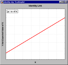
| Identity link: | f(z) = z | |
 | ||
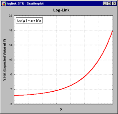
| Log link: | f(z) = log(z) | |
 | ||
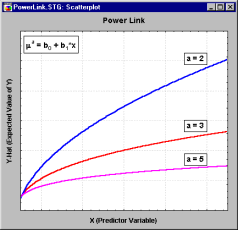
| Power link: | f(z) = za, | for a given a |
 | ||
| Logit link: | f(z)=log(z/(1-z)) | |
| Probit link: | f(z)=invnorm(z) | where invnorm is the inverse of the standard normal cumulative distribution function. |
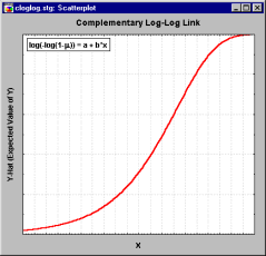
| Complementary log-log link: | f(z)=log(-log(1-z)) | |
 | ||
| Log-log link: | f(z)=-log(-log(z)) | |
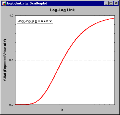 | ||
| Generalized logit link: | f(z1|z2,�,zc)=log(x1/(1-z1-�-zc)) |
| where the model has c+1 categories. | |
Estimation in the generalized linear model. The values of the parameters (b0 through bk and the scale parameter) in the generalized linear model are obtained by maximum likelihood (ML) estimation, which requires iterative computational procedures. There are many iterative methods for ML estimation in the generalized linear model, of which the Newton-Raphson and Fisher-Scoring methods are among the most efficient and widely used (see Dobson,1990). The Fisher-scoring (or iterative re-weighted least squares) method in particular provides a unified algorithm for all generalized linear models, as well as providing the expected variance-covariance matrix of parameter estimates as a byproduct of its computations.
Statistical significance testing Tests for the significance of the effects in the model can be performed via the Wald statistic, the likelihood ratio (LR), or score statistic. Detailed descriptions of these tests can be found in McCullagh and Nelder (1989). The Wald statistic (e.g., see Dobson,1990), which is computed as the generalized inner product of the parameter estimates with the respective variance-covariance matrix, is an easily computed, efficient statistic for testing the significance of effects. The score statistic is obtained from the generalized inner product of the score vector with the Hessian matrix (the matrix of the second-order partial derivatives of the maximum likelihood parameter estimates). The likelihood ratio (LR) test requires the greatest computational effort (another iterative estimation procedure) and is thus not as fast as the first two methods; however, the LR test provides the most asymptotically efficient test known. For details concerning these different test statistics, see Agresti(1996), McCullagh and Nelder(1989), and Dobson(1990).
Diagnostics in the generalized linear model. The two basic types of residuals are the so-called Pearson residuals and deviance residuals. Pearson residuals are based on the difference between observed responses and the predicted values; deviance residuals are based on the contribution of the observed responses to the log-likelihood statistic. In addition, leverage scores, studentized residuals, generalized Cook's D, and other observational statistics (statistics based on individual observations) can be computed. For a description and discussion of these statistics, see Hosmer and Lemeshow (1989).
| To index |
The design for an analysis can include effects for continuous as well as categorical predictor variables. Designs may include polynomials for continuous predictors (e.g., squared or cubic terms) as well as interaction effects (i.e., product terms) for continuous predictors. For categorical predictor variables, one can fit ANOVA-like designs, including full factorial, nested, and fractional factorial designs, etc. Designs can be incomplete (i.e., involve missing cells), and effects for categorical predictor variables can be represented using either the sigma-restricted parameterization or the overparameterized (i.e., indicator variable) representation of effects.
The topics below give complete descriptions of the types of designs that can be analyzed using the generalized linear model, as well as types of designs that can be analyzed using the general linear model.
Signal detection theory. The list of designs shown below is by no means comprehensive, i.e., it does not describe all possible research problems to which the generalized linear model can be applied. For example, an important application of the generalized linear model is the estimation of parameters for Signal detection theory (SDT) models. SDT is an application of statistical decision theory used to detect a signal embedded in noise. SDT is used in psychophysical studies of detection, recognition, and discrimination, and in other areas such as medical research, weather forecasting, survey research, and marketing research. For example, DeCarlo (1998) shows how signal detection models based on different underlying distributions can easily be considered by using the generalized linear model with different link functions.
For discussion of the generalized linear model and the link functions which it uses, see Computational Approaches.
Overview. The levels or values of the predictor variables in an analysis describe the differences between the n subjects or the n valid cases that are analyzed. Thus, when we speak of the between subject design (or simply the between design) for an analysis, we are referring to the nature, number, and arrangement of the predictor variables.
Concerning the nature or type of predictor variables, between designs which contain only categorical predictor variables can be called ANOVA (analysis of variance) designs, between designs which contain only continuous predictor variables can be called regression designs, and between designs which contain both categorical and continuous predictor variables can be called ANCOVA (analysis of covariance) designs. Further, continuous predictors are always considered to have fixed values, but the levels of categorical predictors can be considered to be fixed or to vary randomly. Designs which contain random categorical factors are called mixed-model designs (see the Variance Components and Mixed Model ANOVA/ANCOVA chapter).
Between designs may involve only a single predictor variable and therefore be described as simple (e.g., simple regression) or may employ numerous predictor variables (e.g., multiple regression).
Concerning the arrangement of predictor variables, some between designs employ only "main effect" or first-order terms for predictors, that is, the values for different predictor variables are independent and raised only to the first power. Other between designs may employ higher-order terms for predictors by raising the values for the original predictor variables to a power greater than 1 (e.g., in polynomial regression designs), or by forming products of different predictor variables (i.e., interaction terms). A common arrangement for ANOVA designs is the full-factorial design, in which every combination of levels for each of the categorical predictor variables is represented in the design. Designs with some but not all combinations of levels for each of the categorical predictor variables are aptly called fractional factorial designs. Designs with a hierarchy of combinations of levels for the different categorical predictor variables are called nested designs.
These basic distinctions about the nature, number, and arrangement of predictor variables can be used in describing a variety of different types of between designs. Some of the more common between designs can now be described.
One-Way ANOVA. A design with a single categorical predictor variable is called a one-way ANOVA design. For example, a study of 4 different fertilizers used on different individual plants could be analyzed via one-way ANOVA, with four levels for the factor Fertilizer.
In genera, consider a single categorical predictor variable A with 1 case in each of its 3 categories. Using the sigma-restricted coding of A into 2 quantitative contrast variables, the matrix X defining the between design is

That is, cases in groups A1, A2, and A3 are all assigned values of 1 on X0 (the intercept), the case in group A1 is assigned a value of 1 on X1 and a value 0 on X2, the case in group A2 is assigned a value of 0 on X1 and a value 1 on X2, and the case in group A3 is assigned a value of -1 on X1 and a value -1 on X2. Of course, any additional cases in any of the 3 groups would be coded similarly. If there were 1 case in group A1, 2 cases in group A2, and 1 case in group A3, the X matrix would be

where the first subscript for A gives the replicate number for the cases in each group. For brevity, replicates usually are not shown when describing ANOVA design matrices.
Note that in one-way designs with an equal number of cases in each group, sigma-restricted coding yields X1 � Xk variables all of which have means of 0.
Using the overparameterized model to represent A, the X matrix defining the between design is simply

These simple examples show that the X matrix actually serves two purposes. It specifies (1) the coding for the levels of the original predictor variables on the X variables used in the analysis as well as (2) the nature, number, and arrangement of the X variables, that is, the between design.
Main Effect ANOVA. Main effect ANOVA designs contain separate one-way ANOVA designs for 2 or more categorical predictors. A good example of main effect ANOVA would be the typical analysis performed on screening designs as described in the context of the Experimental Design chapter.
Consider 2 categorical predictor variables A and B each with 2 categories. Using the sigma-restricted coding, the X matrix defining the between design is

Note that if there are equal numbers of cases in each group, the sum of the cross-products of values for the X1 and X2 columns is 0, for example, with 1 case in each group (1*1)+(1*-1)+(-1*1)+(-1*-1)=0. Using the overparameterized model, the matrix X defining the between design is

Comparing the two types of coding, it can be seen that the overparameterized coding takes almost twice as many values as the sigma-restricted coding to convey the same information.
Factorial ANOVA. Factorial ANOVA designs contain X variables representing combinations of the levels of 2 or more categorical predictors (e.g., a study of boys and girls in four age groups, resulting in a 2 (Gender) x 4 (Age Group) design). In particular, full-factorial designs represent all possible combinations of the levels of the categorical predictors. A full-factorial design with 2 categorical predictor variables A and B each with 2 levels each would be called a 2 x 2 full-factorial design. Using the sigma-restricted coding, the X matrix for this design would be
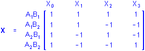
Several features of this X matrix deserve comment. Note that the X1 and X2 columns represent main effect contrasts for one variable, (i.e., A and B, respectively) collapsing across the levels of the other variable. The X3 column instead represents a contrast between different combinations of the levels of A and B. Note also that the values for X3 are products of the corresponding values for X1 and X2. Product variables such as X3 represent the multiplicative or interaction effects of their factors, so X3 would be said to represent the 2-way interaction of A and B. The relationship of such product variables to the dependent variables indicate the interactive influences of the factors on responses above and beyond their independent (i.e., main effect) influences on responses. Thus, factorial designs provide more information about the relationships between categorical predictor variables and responses on the dependent variables than is provided by corresponding one-way or main effect designs.
When many factors are being investigated, however, full-factorial designs sometimes require more data than reasonably can be collected to represent all possible combinations of levels of the factors, and high-order interactions between many factors can become difficult to interpret. With many factors, a useful alternative to the full-factorial design is the fractional factorial design. As an example, consider a 2 x 2 x 2 fractional factorial design to degree 2 with 3 categorical predictor variables each with 2 levels. The design would include the main effects for each variable, and all 2-way interactions between the three variables, but would not include the 3-way interaction between all three variables. Using the overparameterized model, the X matrix for this design is
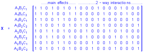
The 2-way interactions are the highest degree effects included in the design. These types of designs are discussed in detail the 2**(k-p) Fractional Factorial Designs section of the Experimental Design chapter.
Nested ANOVA Designs. Nested designs are similar to fractional factorial designs in that all possible combinations of the levels of the categorical predictor variables are not represented in the design. In nested designs, however, the omitted effects are lower-order effects. Nested effects are effects in which the nested variables never appear as main effects. Suppose that for 2 variables A and B with 3 and 2 levels, respectively, the design includes the main effect for A and the effect of B nested within the levels of A. The X matrix for this design using the overparameterized model is
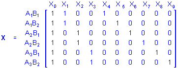
Note that if the sigma-restricted coding were used, there would be only 2 columns in the X matrix for the B nested within A effect instead of the 6 columns in the X matrix for this effect when the overparameterized model coding is used (i.e., columns X4 through X9). The sigma-restricted coding method is overly-restrictive for nested designs, so only the overparameterized model is used to represent nested designs.
Simple Regression. Simple regression designs involve a single continuous predictor variable. If there were 3 cases with values on a predictor variable P of, say, 7, 4, and 9, and the design is for the first-order effect of P, the X matrix would be

and using P for X1 the regression equation would be
Y = b0 + b1P
If the simple regression design is for a higher-order effect of P, say the quadratic effect, the values in the X1 column of the design matrix would be raised to the 2nd power, that is, squared

and using P2 for X1 the regression equation would be
Y = b0 + b1P2
The sigma-restricted and overparameterized coding methods do not apply to simple regression designs and any other design containing only continuous predictors (since there are no categorical predictors to code). Regardless of which coding method is chosen, values on the continuous predictor variables are raised to the desired power and used as the values for the X variables. No recoding is performed. It is therefore sufficient, in describing regression designs, to simply describe the regression equation without explicitly describing the design matrix X.
Multiple Regression. Multiple regression designs are to continuous predictor variables as main effect ANOVA designs are to categorical predictor variables, that is, multiple regression designs contain the separate simple regression designs for 2 or more continuous predictor variables. The regression equation for a multiple regression design for the first-order effects of 3 continuous predictor variables P, Q, and R would be
Y = b0 + b1P + b2Q + b3R
Factorial Regression. Factorial regression designs are similar to factorial ANOVA designs, in which combinations of the levels of the factors are represented in the design. In factorial regression designs, however, there may be many more such possible combinations of distinct levels for the continuous predictor variables than there are cases in the data set. To simplify matters, full-factorial regression designs are defined as designs in which all possible products of the continuous predictor variables are represented in the design. For example, the full-factorial regression design for two continuous predictor variables P and Q would include the main effects (i.e., the first-order effects) of P and Q and their 2-way P by Q interaction effect, which is represented by the product of P and Q scores for each case. The regression equation would be
Y = b0 + b1P + b2Q + b3P*Q
Factorial regression designs can also be fractional, that is, higher-order effects can be omitted from the design. A fractional factorial design to degree 2 for 3 continuous predictor variables P, Q, and R would include the main effects and all 2-way interactions between the predictor variables
Y = b0 + b1P + b2Q + b3R + b4P*Q + b5P*R + b6Q*R
Polynomial Regression. Polynomial regression designs are designs which contain main effects and higher-order effects for the continuous predictor variables but do not include interaction effects between predictor variables. For example, the polynomial regression design to degree 2 for three continuous predictor variables P, Q, and R would include the main effects (i.e., the first-order effects) of P, Q, and R and their quadratic (i.e., second-order) effects, but not the 2-way interaction effects or the P by Q by R 3-way interaction effect.
Y = b0 + b1P + b2P2 + b3Q + b4Q2 + b5R + b6R2
Polynomial regression designs do not have to contain all effects up to the same degree for every predictor variable. For example, main, quadratic, and cubic effects could be included in the design for some predictor variables, and effects up the fourth degree could be included in the design for other predictor variables.
Response Surface Regression. Quadratic response surface regression designs are a hybrid type of design with characteristics of both polynomial regression designs and fractional factorial regression designs. Quadratic response surface regression designs contain all the same effects of polynomial regression designs to degree 2 and additionally the 2-way interaction effects of the predictor variables. The regression equation for a quadratic response surface regression design for 3 continuous predictor variables P, Q, and R would be
Y = b0 + b1P + b2P2 + b3Q + b4Q2 + b5R + b6R2 + b7P*Q + b8P*R + b9Q*R
These types of designs are commonly employed in applied research (e.g., in industrial experimation), and a detailed discussion of these types of designs is also presented in the Experimental Design chapter (see Central composite designs).
Mixture Surface Regression. Mixture surface regression designs are identical to factorial regression designs to degree 2 except for the omission of the intercept. Mixtures, as the name implies, add up to a constant value; the sum of the proportions of ingredients in different recipes for some material all must add up 100%. Thus, the proportion of one ingredient in a material is redundant with the remaining ingredients. Mixture surface regression designs deal with this redundancy by omitting the intercept from the design. The design matrix for a mixture surface regression design for 3 continuous predictor variables P, Q, and R would be
Y = b1P + b2Q + b3R + b4P*Q + b5P*R + b6Q*R
These types of designs are commonly employed in applied research (e.g., in industrial experimation), and a detailed discussion of these types of designs is also presented in the Experimental Design chapter (see Mixture designs and triangular surfaces).
Analysis of Covariance. In general, between designs which contain both categorical and continuous predictor variables can be called ANCOVA designs. Traditionally, however, ANCOVA designs have referred more specifically to designs in which the first-order effects of one or more continuous predictor variables are taken into account when assessing the effects of one or more categorical predictor variables. A basic introduction to analysis of covariance can also be found in the Analysis of covariance (ANCOVA) topic of the ANOVA/MANOVA chapter.
To illustrate, suppose a researcher wants to assess the influences of a categorical predictor variable A with 3 levels on some outcome, and that measurements on a continuous predictor variable P, known to covary with the outcome, are available. If the data for the analysis are

then the sigma-restricted X matrix for the design that includes the separate first-order effects of P and A would be
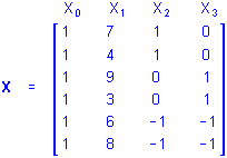
The b2 and b3 coefficients in the regression equation
Y = b0 + b1X1 + b2X2 + b3X3
represent the influences of group membership on the A categorical predictor variable, controlling for the influence of scores on the P continuous predictor variable. Similarly, the b1 coefficient represents the influence of scores on P controlling for the influences of group membership on A. This traditional ANCOVA analysis gives a more sensitive test of the influence of A to the extent that P reduces the prediction error, that is, the residuals for the outcome variable.
The X matrix for the same design using the overparameterized model would be
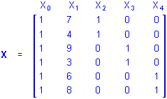
The interpretation is unchanged except that the influences of group membership on the A categorical predictor variables are represented by the b2, b3 and b4 coefficients in the regression equation
Y = b0 + b1X1 + b2X2 + b3X3 + b4X4
Separate Slope Designs. The traditional analysis of covariance (ANCOVA) design for categorical and continuous predictor variables is inappropriate when the categorical and continuous predictors interact in influencing responses on the outcome. The appropriate design for modeling the influences of the predictors in this situation is called the separate slope design. For the same example data used to illustrate traditional ANCOVA, the overparameterized X matrix for the design that includes the main effect of the three-level categorical predictor A and the 2-way interaction of P by A would be
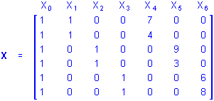
The b4, b5, and b6 coefficients in the regression equation
Y = b0 + b1X1 + b2X2 + b3X3 + b4X4 + b5X5 + b6X6
give the separate slopes for the regression of the outcome on P within each group on A, controlling for the main effect of A.
As with nested ANOVA designs, the sigma-restricted coding of effects for separate slope designs is overly restrictive, so only the overparameterized model is used to represent separate slope designs. In fact, separate slope designs are identical in form to nested ANOVA designs, since the main effects for continuous predictors are omitted in separate slope designs.
Homogeneity of Slopes. The appropriate design for modeling the influences of continuous and categorical predictor variables depends on whether the continuous and categorical predictors interact in influencing the outcome. The traditional analysis of covariance (ANCOVA) design for continuous and categorical predictor variables is appropriate when the continuous and categorical predictors do not interact in influencing responses on the outcome, and the separate slope design is appropriate when the continuous and categorical predictors do interact in influencing responses. The homogeneity of slopes designs can be used to test whether the continuous and categorical predictors interact in influencing responses, and thus, whether the traditional ANCOVA design or the separate slope design is appropriate for modeling the effects of the predictors. For the same example data used to illustrate the traditional ANCOVA and separate slope designs, the overparameterized X matrix for the design that includes the main effect of P, the main effect of the three-level categorical predictor A, and the 2-way interaction of P by A would be
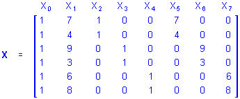
If the b5, b6, or b7 coefficient in the regression equation
Y = b0 + b1X1 + b2X2 + b3X3 + b4X4 + b5X5 + b6X6 + b7X7
is non-zero, the separate slope model should be used. If instead all 3 of these regression coefficients are zero the traditional ANCOVA design should be used.
The sigma-restricted X matrix for the homogeneity of slopes design would be
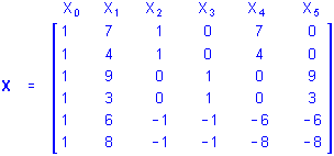
Using this X matrix, if the b4, or b5 coefficient in the regression equation
Y = b0 + b1X1 + b2X2 + b3X3 + b4X4 + b5X5
is non-zero, the separate slope model should be used. If instead both of these regression coefficients are zero the traditional ANCOVA design should be used.
| To index |
In addition to fitting the whole model for the specified type of analysis, different methods for automatic model building can be employed in analyses using the generalized linear model. Specifically, forward entry, backward removal, forward stepwise, and backward stepwise procedures can be performed, as well as best-subset search procedures. In forward methods of selection of effects to include in the model (i.e., forward entry and forward stepwise methods), score statistics are compared to select new (significant) effects. The Wald statistic can be used for backward removal methods (i.e., backward removal and backward stepwise, when effects are selected for removal from the model).
The best subsets search method can be based on three different test statistics: the score statistic, the model likelihood, and the AIC (Akaike Information Criterion, see Akaike, 1973). Note that, since the score statistic does not require iterative computations, best subset selection based on the score statistic is computationally fastest, while selection based on the other two statistics usually provides more accurate results; see McCullagh and Nelder(1989), for additional details.
| To index |
Simple estimation and test statistics may not be sufficient for adequate interpretation of the effects in an analysis. Especially for higher order (e.g., interaction) effects, inspection of the observed and predicted means can be invaluable for understanding the nature of an effect. Plots of these means (with error bars) can be useful for quickly grasping the role of the effects in the model.
Inspection of the distributions of variables is critically important when using the generalized linear model. Histograms and probability plots for variables, and scatterplots showing the relationships between observed values, predicted values, and residuals (e.g., Pearson residuals, deviance residuals, studentized residuals, differential Chi-square statistics, differential deviance statistics, and generalized Cook's D) provide invaluable model-checking tools.
| To index |
