This chapter describes the use of partial least squares regression analysis. If you are unfamiliar with the basic methods of regression in linear models, it may be useful to first review the basic information on these topics in Elementary Concepts the different designs discussed in this chapter are also described in the context of General Linear Models, Generalized Linear Models, and General Stepwise Regression.
Y = b0 + b1X1 + b2X2 + ... + bpXp
In this equation b0 is the regression coefficient for the intercept and the bi values are the regression coefficients (for variables 1 through p) computed from the data.
So for example, one could estimate (i.e., predict) a person's weight as a function of the person's height and gender. You could use linear regression to estimate the respective regression coefficients from a sample of data, measuring height, weight, and observing the subjects' gender. For many data analysis problems, estimates of the linear relationships between variables are adequate to describe the observed data, and to make reasonable predictions for new observations (see Multiple Regression or General Stepwise Regression for additional details).
The multiple linear regression model has been extended in a number of ways to address more sophisticated data analysis problems. The multiple linear regression model serves as the basis for a number of multivariate methods such as discriminant analysis (i.e., the prediction of group membership from the levels of continuous predictor variables), principal components regression (i.e., the prediction of responses on the dependent variables from factors underlying the levels of the predictor variables), and canonical correlation (i.e., the prediction of factors underlying responses on the dependent variables from factors underlying the levels of the predictor variables). These multivariate methods all have two important properties in common. These methods impose restrictions such that (1) factors underlying the Y and X variables are extracted from the Y'Y and X'X matrices, respectively, and never from cross-product matrices involving both the Y and X variables, and (2) the number of prediction functions can never exceed the minimum of the number of Y variables and X variables.
Partial least squares regression extends multiple linear regression without imposing the restrictions employed by discriminant analysis, principal components regression, and canonical correlation. In partial least squares regression, prediction functions are represented by factors extracted from the Y'XX'Y matrix. The number of such prediction functions that can be extracted typically will exceed the maximum of the number of Y and X variables.
In short, partial least squares regression is probably the least restrictive of the various multivariate extensions of the multiple linear regression model. This flexibility allows it to be used in situations where the use of traditional multivariate methods is severely limited, such as when there are fewer observations than predictor variables. Furthermore, partial least squares regression can be used as an exploratory analysis tool to select suitable predictor variables and to identify outliers before classical linear regression.
Partial least squares regression has been used in various disciplines such as chemistry, economics, medicine, psychology, and pharmaceutical science where predictive linear modeling, especially with a large number of predictors, is necessary. Especially in chemometrics, partial least squares regression has become a standard tool for modeling linear relations between multivariate measurements (de Jong, 1993).
| To index |
As in multiple linear regression, the main purpose of partial least squares regression is to build a linear model, Y=XB+E, where Y is an n cases by m variables response matrix, X is an n cases by p variables predictor (design) matrix, B is a p by m regression coefficient matrix, and E is a noise term for the model which has the same dimensions as Y. Usually, the variables in X and Y are centered by subtracting their means and scaled by dividing by their standard deviations. For more information about centering and scaling in partial least squares regression, you can refer to Geladi and Kowalsky(1986).
Both principal components regression and partial least squares regression produce factor scores as linear combinations of the original predictor variables, so that there is no correlation between the factor score variables used in the predictive regression model. For example, suppose we have a data set with response variables Y (in matrix form) and a large number of predictor variables X (in matrix form), some of which are highly correlated. A regression using factor extraction for this type of data computes the factor score matrix T=XW for an appropriate weight matrix W, and then considers the linear regression model Y=TQ+E, where Q is a matrix of regression coefficients (loadings) for T, and E is an error (noise) term. Once the loadings Q are computed, the above regression model is equivalent to Y=XB+E, where B=WQ, which can be used as a predictive regression model.
Principal components regression and partial least squares regression differ in the methods used in extracting factor scores. In short, principal components regression produces the weight matrix W reflecting the covariance structure between the predictor variables, while partial least squares regression produces the weight matrix W reflecting the covariance structure between the predictor and response variables.
For establishing the model, partial least squares regression produces a p by c weight matrix W for X such that T=XW, i.e., the columns of W are weight vectors for the X columns producing the corresponding n by c factor score matrix T. These weights are computed so that each of them maximizes the covariance between responses and the corresponding factor scores. Ordinary least squares procedures for the regression of Y on T are then performed to produce Q, the loadings for Y (or weights for Y) such that Y=TQ+E. Once Q is computed, we have Y=XB+E, where B=WQ, and the prediction model is complete.
One additional matrix which is necessary for a complete description of partial least squares regression procedures is the p by c factor loading matrix P which gives a factor model X=TP+F, where F is the unexplained part of the X scores. We now can describe the algorithms for computing partial least squares regression.
The standard algorithm for computing partial least squares regression components (i.e., factors) is nonlinear iterative partial least squares (NIPALS). There are many variants of the NIPALS algorithm which normalize or do not normalize certain vectors. The following algorithm, which assumes that the X and Y variables have been transformed to have means of zero, is considered to be one of most efficient NIPALS algorithms.
For each h=1,�,c, where A0=X'Y, M0=X'X, C0=I, and c given,
An alternative estimation method for partial least squares regression components is the SIMPLS algorithm (de Jong, 1993), which can be described as follows.
For each h=1,�,c, where A0=X'Y, M0=X'X, C0=I, and c given,
| To index |
A very important step when fitting models to be used for prediction of future observation is to verify (cross-validate) the results, i.e., to apply the current results to a new set of observations that was not used to compute those results (estimate the parameters). Some software programs offer very flexible methods for computing detailed predicted value and residual statistics for observations (1) that were not used in the computations for fitting the current model and have observed values for the dependent variables (the so-called cross-validation sample), and (2) that were not used in the computations for fitting the current model, and have missing data for the dependent variables (prediction sample.
| To index |
The design for an analysis can include effects for continuous as well as categorical predictor variables. Designs may include polynomials for continuous predictors (e.g., squared or cubic terms) as well as interaction effects (i.e., product terms) for continuous predictors. For categorical predictor, one can fit ANOVA-like designs, including full factorial, nested, and fractional factorial designs, etc. Designs can be incomplete (i.e., involve missing cells), and effects for categorical predictor variables can be represented using either the sigma-restricted parameterization or the overparameterized (i.e., indicator variable) representation of effects.
The topics below give complete descriptions of the types of designs that can be analyzed using partial least squares regression, as well as types of designs that can be analyzed using the general linear model.
Overview. The levels or values of the predictor variables in an analysis describe the differences between the n subjects or the n valid cases that are analyzed. Thus, when we speak of the between subject design (or simply the between design) for an analysis, we are referring to the nature, number, and arrangement of the predictor variables.
Concerning the nature or type of predictor variables, between designs which contain only categorical predictor variables can be called ANOVA (analysis of variance) designs, between designs which contain only continuous predictor variables can be called regression designs, and between designs which contain both categorical and continuous predictor variables can be called ANCOVA (analysis of covariance) designs. Further, continuous predictors are always considered to have fixed values, but the levels of categorical predictors can be considered to be fixed or to vary randomly. Designs which contain random categorical factors are called mixed-model designs (see the Variance Components and Mixed Model ANOVA/ANCOVA chapter).
Between designs may involve only a single predictor variable and therefore be described as simple (e.g., simple regression) or may employ numerous predictor variables (e.g., multiple regression).
Concerning the arrangement of predictor variables, some between designs employ only "main effect" or first-order terms for predictors, that is, the values for different predictor variables are independent and raised only to the first power. Other between designs may employ higher-order terms for predictors by raising the values for the original predictor variables to a power greater than 1 (e.g., in polynomial regression designs), or by forming products of different predictor variables (i.e., interaction terms). A common arrangement for ANOVA designs is the full-factorial design, in which every combination of levels for each of the categorical predictor variables is represented in the design. Designs with some but not all combinations of levels for each of the categorical predictor variables are aptly called fractional factorial designs. Designs with a hierarchy of combinations of levels for the different categorical predictor variables are called nested designs.
These basic distinctions about the nature, number, and arrangement of predictor variables can be used in describing a variety of different types of between designs. Some of the more common between designs can now be described.
One-Way ANOVA. A design with a single categorical predictor variable is called a one-way ANOVA design. For example, a study of 4 different fertilizers used on different individual plants could be analyzed via one-way ANOVA, with four levels for the factor Fertilizer.
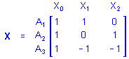
In genera, consider a single categorical predictor variable A with 1 case in each of its 3 categories. Using the sigma-restricted coding of A into 2 quantitative contrast variables, the matrix X defining the between design is
That is, cases in groups A1, A2, and A3 are all assigned values of 1 on X0 (the intercept), the case in group A1 is assigned a value of 1 on X1 and a value 0 on X2, the case in group A2 is assigned a value of 0 on X1 and a value 1 on X2, and the case in group A3 is assigned a value of -1 on X1 and a value -1 on X2. Of course, any additional cases in any of the 3 groups would be coded similarly. If there were 1 case in group A1, 2 cases in group A2, and 1 case in group A3, the X matrix would be
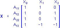
where the first subscript for A gives the replicate number for the cases in each group. For brevity, replicates usually are not shown when describing ANOVA design matrices.
Note that in one-way designs with an equal number of cases in each group, sigma-restricted coding yields X1 � Xk variables all of which have means of 0.
Using the overparameterized model to represent A, the X matrix defining the between design is simply
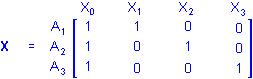
These simple examples show that the X matrix actually serves two purposes. It specifies (1) the coding for the levels of the original predictor variables on the X variables used in the analysis as well as (2) the nature, number, and arrangement of the X variables, that is, the between design.
Main Effect ANOVA. Main effect ANOVA designs contain separate one-way ANOVA designs for 2 or more categorical predictors. A good example of main effect ANOVA would be the typical analysis performed on screening designs as described in the context of the Experimental Design chapter.
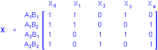
Consider 2 categorical predictor variables A and B each with 2 categories. Using the sigma-restricted coding, the X matrix defining the between design is
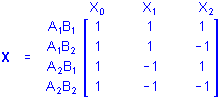
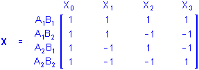
Note that if there are equal numbers of cases in each group, the sum of the cross-products of values for the X1 and X2 columns is 0, for example, with 1 case in each group (1*1)+(1*-1)+(-1*1)+(-1*-1)=0. Using the overparameterized model, the matrix X defining the between design is
Comparing the two types of coding, it can be seen that the overparameterized coding takes almost twice as many values as the sigma-restricted coding to convey the same information.
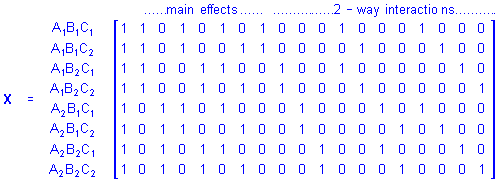
Factorial ANOVA. Factorial ANOVA designs contain X variables representing combinations of the levels of 2 or more categorical predictors (e.g., a study of boys and girls in four age groups, resulting in a 2 (Gender) x 4 (Age Group) design). In particular, full-factorial designs represent all possible combinations of the levels of the categorical predictors. A full-factorial design with 2 categorical predictor variables A and B each with 2 levels each would be called a 2 x 2 full-factorial design. Using the sigma-restricted coding, the X matrix for this design would be
Several features of this X matrix deserve comment. Note that the X1 and X2 columns represent main effect contrasts for one variable, (i.e., A and B, respectively) collapsing across the levels of the other variable. The X3 column instead represents a contrast between different combinations of the levels of A and B. Note also that the values for X3 are products of the corresponding values for X1 and X2. Product variables such as X3 represent the multiplicative or interaction effects of their factors, so X3 would be said to represent the 2-way interaction of A and B. The relationship of such product variables to the dependent variables indicate the interactive influences of the factors on responses above and beyond their independent (i.e., main effect) influences on responses. Thus, factorial designs provide more information about the relationships between categorical predictor variables and responses on the dependent variables than is provided by corresponding one-way or main effect designs.
When many factors are being investigated, however, full-factorial designs sometimes require more data than reasonably can be collected to represent all possible combinations of levels of the factors, and high-order interactions between many factors can become difficult to interpret. With many factors, a useful alternative to the full-factorial design is the fractional factorial design. As an example, consider a 2 x 2 x 2 fractional factorial design to degree 2 with 3 categorical predictor variables each with 2 levels. The design would include the main effects for each variable, and all 2-way interactions between the three variables, but would not include the 3-way interaction between all three variables. Using the overparameterized model, the X matrix for this design is
The 2-way interactions are the highest degree effects included in the design. These types of designs are discussed in detail the 2**(k-p) Fractional Factorial Designs section of the Experimental Design chapter.
Nested ANOVA Designs. Nested designs are similar to fractional factorial designs in that all possible combinations of the levels of the categorical predictor variables are not represented in the design. In nested designs, however, the omitted effects are lower-order effects. Nested effects are effects in which the nested variables never appear as main effects. Suppose that for 2 variables A and B with 3 and 2 levels, respectively, the design includes the main effect for A and the effect of B nested within the levels of A. The X matrix for this design using the overparameterized model is
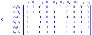
Note that if the sigma-restricted coding were used, there would be only 2 columns in the X matrix for the B nested within A effect instead of the 6 columns in the X matrix for this effect when the overparameterized model coding is used (i.e., columns X4 through X9). The sigma-restricted coding method is overly-restrictive for nested designs, so only the overparameterized model is used to represent nested designs.
Simple Regression. Simple regression designs involve a single continuous predictor variable. If there were 3 cases with values on a predictor variable P of, say, 7, 4, and 9, and the design is for the first-order effect of P, the X matrix would be
and using P for X1 the regression equation would be
Y = b0 + b1P
If the simple regression design is for a higher-order effect of P, say the quadratic effect, the values in the X1 column of the design matrix would be raised to the 2nd power, that is, squared
and using P2 for X1 the regression equation would be
Y = b0 + b1P2
The sigma-restricted and overparameterized coding methods do not apply to simple regression designs and any other design containing only continuous predictors (since there are no categorical predictors to code). Regardless of which coding method is chosen, values on the continuous predictor variables are raised to the desired power and used as the values for the X variables. No recoding is performed. It is therefore sufficient, in describing regression designs, to simply describe the regression equation without explicitly describing the design matrix X.
Multiple Regression. Multiple regression designs are to continuous predictor variables as main effect ANOVA designs are to categorical predictor variables, that is, multiple regression designs contain the separate simple regression designs for 2 or more continuous predictor variables. The regression equation for a multiple regression design for the first-order effects of 3 continuous predictor variables P, Q, and R would be
Y = b0 + b1P + b2Q + b3R
Factorial Regression. Factorial regression designs are similar to factorial ANOVA designs, in which combinations of the levels of the factors are represented in the design. In factorial regression designs, however, there may be many more such possible combinations of distinct levels for the continuous predictor variables than there are cases in the data set. To simplify matters, full-factorial regression designs are defined as designs in which all possible products of the continuous predictor variables are represented in the design. For example, the full-factorial regression design for two continuous predictor variables P and Q would include the main effects (i.e., the first-order effects) of P and Q and their 2-way P by Q interaction effect, which is represented by the product of P and Q scores for each case. The regression equation would be
Y = b0 + b1P + b2Q + b3P*Q
Factorial regression designs can also be fractional, that is, higher-order effects can be omitted from the design. A fractional factorial design to degree 2 for 3 continuous predictor variables P, Q, and R would include the main effects and all 2-way interactions between the predictor variables
Y = b0 + b1P + b2Q + b3R + b4P*Q + b5P*R + b6Q*R
Polynomial Regression. Polynomial regression designs are designs which contain main effects and higher-order effects for the continuous predictor variables but do not include interaction effects between predictor variables. For example, the polynomial regression design to degree 2 for three continuous predictor variables P, Q, and R would include the main effects (i.e., the first-order effects) of P, Q, and R and their quadratic (i.e., second-order) effects, but not the 2-way interaction effects or the P by Q by R 3-way interaction effect.
Y = b0 + b1P + b2P2 + b3Q + b4Q2 + b5R + b6R2
Polynomial regression designs do not have to contain all effects up to the same degree for every predictor variable. For example, main, quadratic, and cubic effects could be included in the design for some predictor variables, and effects up the fourth degree could be included in the design for other predictor variables.
Response Surface Regression. Quadratic response surface regression designs are a hybrid type of design with characteristics of both polynomial regression designs and fractional factorial regression designs. Quadratic response surface regression designs contain all the same effects of polynomial regression designs to degree 2 and additionally the 2-way interaction effects of the predictor variables. The regression equation for a quadratic response surface regression design for 3 continuous predictor variables P, Q, and R would be
Y = b0 + b1P + b2P2 + b3Q + b4Q2 + b5R + b6R2 + b7P*Q + b8P*R + b9Q*R
These types of designs are commonly employed in applied research (e.g., in industrial experimation), and a detailed discussion of these types of designs is also presented in the Experimental Design chapter (see Central composite designs).
Analysis of Covariance. In general, between designs which contain both categorical and continuous predictor variables can be called ANCOVA designs. Traditionally, however, ANCOVA designs have referred more specifically to designs in which the first-order effects of one or more continuous predictor variables are taken into account when assessing the effects of one or more categorical predictor variables. A basic introduction to analysis of covariance can also be found in the Analysis of covariance (ANCOVA) topic of the ANOVA/MANOVA chapter.
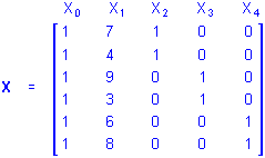
To illustrate, suppose a researcher wants to assess the influences of a categorical predictor variable A with 3 levels on some outcome, and that measurements on a continuous predictor variable P, known to covary with the outcome, are available. If the data for the analysis are
then the sigma-restricted X matrix for the design that includes the separate first-order effects of P and A would be
The b2 and b3 coefficients in the regression equation
Y = b0 + b1X1 + b2X2 + b3X3
represent the influences of group membership on the A categorical predictor variable, controlling for the influence of scores on the P continuous predictor variable. Similarly, the b1 coefficient represents the influence of scores on P controlling for the influences of group membership on A. This traditional ANCOVA analysis gives a more sensitive test of the influence of A to the extent that P reduces the prediction error, that is, the residuals for the outcome variable.
The X matrix for the same design using the overparameterized model would be
The interpretation is unchanged except that the influences of group membership on the A categorical predictor variables are represented by the b2, b3 and b4 coefficients in the regression equation
Y = b0 + b1X1 + b2X2 + b3X3 + b4X4
Separate Slope Designs. The traditional analysis of covariance (ANCOVA) design for categorical and continuous predictor variables is inappropriate when the categorical and continuous predictors interact in influencing responses on the outcome. The appropriate design for modeling the influences of the predictors in this situation is called the separate slope design. For the same example data used to illustrate traditional ANCOVA, the overparameterized X matrix for the design that includes the main effect of the three-level categorical predictor A and the 2-way interaction of P by A would be
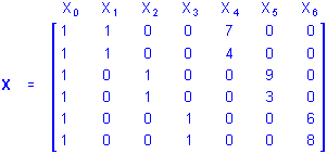
The b4, b5, and b6 coefficients in the regression equation
Y = b0 + b1X1 + b2X2 + b3X3 + b4X4 + b5X5 + b6X6
give the separate slopes for the regression of the outcome on P within each group on A, controlling for the main effect of A.
As with nested ANOVA designs, the sigma-restricted coding of effects for separate slope designs is overly restrictive, so only the overparameterized model is used to represent separate slope designs. In fact, separate slope designs are identical in form to nested ANOVA designs, since the main effects for continuous predictors are omitted in separate slope designs.
Homogeneity of Slopes. The appropriate design for modeling the influences of continuous and categorical predictor variables depends on whether the continuous and categorical predictors interact in influencing the outcome. The traditional analysis of covariance (ANCOVA) design for continuous and categorical predictor variables is appropriate when the continuous and categorical predictors do not interact in influencing responses on the outcome, and the separate slope design is appropriate when the continuous and categorical predictors do interact in influencing responses. The homogeneity of slopes designs can be used to test whether the continuous and categorical predictors interact in influencing responses, and thus, whether the traditional ANCOVA design or the separate slope design is appropriate for modeling the effects of the predictors. For the same example data used to illustrate the traditional ANCOVA and separate slope designs, the overparameterized X matrix for the design that includes the main effect of P, the main effect of the three-level categorical predictor A, and the 2-way interaction of P by A would be
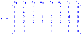
If the b5, b6, or b7 coefficient in the regression equation
Y = b0 + b1X1 + b2X2 + b3X3 + b4X4 + b5X5 + b6X6 + b7X7
is non-zero, the separate slope model should be used. If instead all 3 of these regression coefficients are zero the traditional ANCOVA design should be used.
The sigma-restricted X matrix for the homogeneity of slopes design would be
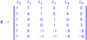
Using this X matrix, if the b4, or b5 coefficient in the regression equation
Y = b0 + b1X1 + b2X2 + b3X3 + b4X4 + b5X5
is non-zero, the separate slope model should be used. If instead both of these regression coefficients are zero the traditional ANCOVA design should be used.
A graphic technique that is useful in analyzing Partial Least Squares designs is a distance graph. These graphs allow you to compute and plot distances from the origin (zero for all dimensions) for the predicted and residual statistics, loadings, and weights for the respective number of components.

Based on Euclidean distances, these observation plots can be helpful in determining major contributors to the prediction of the conceptual variable(s) (plotting weights) as well as outliers that have a disproportionate influence (relative to the other observation) on the results (plotting residual values).
| To index |
