 *j/p) (for j=0 to p)
w-j = wj (for j
 0)
0)
Hamming Window. In Time Series, the Hamming window is a weighted moving average transformation used to smooth the periodogram values. In the Hamming (named after R. W. Hamming) window or Tukey- Hamming window (Blackman and Tukey, 1958), for each frequency, the weights for the weighted moving average of the periodogram values are computed as:
wj = 0.54 + 0.46*cosine(*j/p) (for j=0 to p)
w-j = wj (for j 0)
where p = (m-1)/2
This weight function will assign the greatest weight to the observation being smoothed in the center of the window, and increasingly smaller weights to values that are further away from the center.
See also, Basic Notations and Principles.
Hanging Bars Histogram. The hanging bars histogram offers a "visual test of normality" of the distribution that helps identify the areas of the distribution where the discrepancies (between the observed and expected normal frequencies) occur. While the standard way of presenting the normal distribution fitted to an observed distribution is to overlay the best-fitting normal curve over a histogram, the hanging bars histogram does just the opposite: it suspends the bars representing the observed frequencies for consecutive ranges of values from the best-fitting normal curve.
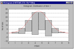
If the investigated distribution can be well approximated by the normal curve, then the bottoms of all bars should form a straight, horizontal line.
Harmonic Mean. The Harmonic Mean is a "summary" statistic used in analyses of frequency data; it is computed as:
H = n * 1/ (1/xi)
where
n is the sample size.
Hazard. It is often meaningful to consider the function that describes the probability of failure during a very small time increment (assuming that no failures have occurred prior to that time). This function is called the hazard function (or, sometimes, also conditional failure, intensity, or force of mortality function), and is generally defined as:
h(t) = f(t)/(1-F(t))
where h(t) stands for the hazard function (of time t), and f(t) and F(t) are the probability density and cumulative distribution functions, respectively.
For additional information see the Survival Analysis chapter, or the Weibull and Reliability/Failure Time Analysis section in the Process Analysis chapter.
Hazard Rate. In Survival Analysis the hazard rate is defined as the probability per time unit that a case that has survived to the beginning of the respective interval will fail in that interval. Specifically, it is computed as the number of failures per time units in the respective interval, divided by the average number of surviving cases at the mid-point of the interval.
Heuristic. As opposed to an algorithm (which contains a fully defined set of steps that will produce a specific outcome), heuristics are general recommendations or guides based on statistical evidence (e.g., "quit smoking to prolong your life," "males with college education are more likely to respond positively to this advertisement than�") or theoretical reasoning (e.g., "the mechanism of the vitamin X synthesis as we understand it, implies that eating Y will reduce the deficit of X"). For more information about the concept of heuristic, see Kahneman, Slovic, & Tversky, 1982.
See also, Data Mining, Neural Networks, algorithm.
Heywood Case. A Heywood case in common factor analysis occurs when the minimum of the discrepancy function is obtained with one or more negative values as estimates for the variance of the unique variables. Such values are of course impossible. Heywood cases occur frequently when too many factors are extracted, or the sample size is too small.
Hidden Layers (in Neural Networks). All layers of a neural network except the input and output layers. Hidden layers provide the network's non-linear modeling capabilities.
High-Low Close. In this type of box or range plot, the "serifs" on the whiskers are not symmetrical but point to the left of the bar, representing the traditional "stock price graph" style. Note that you can change the whisker style (i.e., Hi/Lo Left, Hi/Lo Right, or Whiskers), for example:

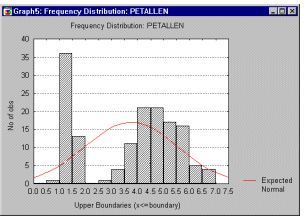
Histograms, 2D. 2D histograms (the term was first used by Pearson, 1895) present a graphical representation (see below) of the frequency distribution of the selected variable(s) in which the columns are drawn over the class intervals and the heights of the columns are proportional to the class frequencies.
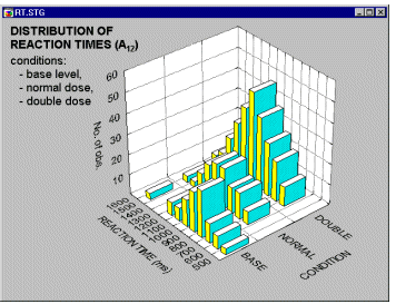
Histograms, 3D Bivariate. Three-dimensional histograms are used to visualize crosstabulations of values in two variables. They can be considered to be a conjunction of two simple (i.e., univariate) histograms, combined such that the frequencies of co-occurrences of values on the two analyzed variables can be examined. In a most common format of this graph, a 3D bar is drawn for each "cell" of the crosstabulation table and the height of the bar represents the frequency of values for the respective cell of the table. Different methods of categorization can be used for each of the two variables for which the bivariate distribution is visualized (see below).
For information on smoothing 3D Bivariate Histograms, see Smoothing Bivariate Distributions.
Histograms, 3D - Box Plots. This type of bivariate histogram represents the frequencies as a series of 3D bars ("rectangular boxes"). This is the default representation of 3D histograms. The "height" of each bar on the Z- axis corresponds to the frequency of the respective combination of levels for the two variables.
Histograms, 3D - Contour/Discrete. This contour plot represents a discrete projection of the 3D (smoothed) histogram.
Histograms, 3D - Contour Plot. This contour plot presents a projection of the spline-smoothed surface fit to the frequency data (see 3D Sequential Surface Plot. Successive values of each series are plotted along the X-axis, with each successive series represented along the Y-axis.
Histograms, 3D - Spikes. In this type of bivariate histogram, the frequencies are represented as a series of "spikes" (point symbols with lines descending to the base plane). The "height" of each spike is determined by the frequency for the respective combination of levels of the two variables.
Histograms, 3D - Surface Plot. In this representaion of the 3D bivariate histogram, a spline-smoothed surface is fit to the frequency data.
Hollander-Proschan Test. This test compares the theoretical reliability function to the Kaplan-Meier estimate. The actual computations for this test are somewhat complex, and you may refer to Dodson (1994, Chapter 4) for a detailed description of the computational formulas. The Hollander-Proschan test is applicable to complete, single-censored, and multiple-censored data sets; however, Dodson (1994) cautions that the test may sometimes indicate a poor fit when the data are heavily single-censored. The Hollander-Proschan C statistic can be tested against the normal distribution (z).
The Hollander-Proschan test is used in Weibull and Reliability/Failure Time Analysis; see also, Mann-Scheuer-Fertig Test and Anderson-Darling Test.
Hooke-Jeeves Pattern Moves. A Nonlinear Estimation procedure which at each iteration, first defines a pattern of points by moving each parameter one by one, so as to optimize the current loss function. The entire pattern of points is then shifted or moved to a new location; this new location is determined by extrapolating the line from the old base point in the m dimensional parameter space to the new base point. The step sizes in this process are constantly adjusted to "zero in" on the respective optimum. This method is usually quite effective, and should be tried if both the quasi-Newton and Simplex methods fail to produce reasonable estimates.
HTM. A file name extension used to save HTML documents (see HTML).
HTML. Acronym for HyperText Markup Language. The markup language used for documents on the World Wide Web. HTML uses tags to identify elements of the document, such as text or graphics. HTML 2.0, defined by the Internet Engineering Task Force (IETF), includes features of HTML common to all Web browsers as of 1995 and was the first version of HTML widely used on the World Wide Web. Future HTML development will be carried out by the World Wide Web Consortium (W3C). HTML 3.2, the latest proposed standard, incorporates features widely implemented as of early 1996. Most Web browsers, notably Netscape Navigator and Internet Explorer, recognize HTML tags beyond those included in the present standard.
Hyperbolic tangent (tanh). A symmetric S-shaped (sigmoid) function, sometimes used as an alternative to logistic functions.
Hyperplane. An N-dimensional analogy of a line or plane, which divides an N+1 dimensional space into two. See, Neural Networks.
Hypersphere. An N-dimensional analogy of a circle or sphere. See, Neural Networks.
