Discrete Distributions |
A random vector X taking values in a countable subset S of Rn is said to be discrete. The (discrete) probability density function of X is the function f from S to R defined by
f(x) = P(X = x) for x in S
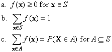
![]() 1. Show that f
satisfies the following properties:
1. Show that f
satisfies the following properties:

Property c is particularly important since it shows that the probability distribution of a discrete random variable is completely determined by its density function. Conversely, any function that satisfies properties a and b is a (discrete) density, and then property c can be used to construct a discrete probability distribution on S.
We can extend f, if we want to, to all of Rn by defining f(x) = 0 for x not in S. Sometimes this extension simplifies formulas and notation.
A vector x in S that maximizes the density f is called a mode of the distribution. When there is only one mode, it is sometimes used as a measure of the center of the distribution.
![]() 2. Suppose that r
is a nonnegative function defined on a countable set S
of Rn and that
2. Suppose that r
is a nonnegative function defined on a countable set S
of Rn and that
Define f(x) = r(x) / c for x in S. Show that f is a discrete density function on S:
The constant c in Exercise 2 is sometimes called the normalizing constant. This result is useful for constructing density functions with desired functional properties (domain, shape, symmetry, and so on). The following exercises describe a very important class of discrete distributions.
![]() 3. Let r(x)
= x2 for x in {-2, -1, 0, 1, 2}.
3. Let r(x)
= x2 for x in {-2, -1, 0, 1, 2}.
![]() 4. Let r(n)
= qn for n = 0, 1, 2, ...
where q is a parameter in (0,1).
4. Let r(n)
= qn for n = 0, 1, 2, ...
where q is a parameter in (0,1).
![]() 5. Let r(i,
j) = i + j for (i, j)
in {0, 1, 2}2.
5. Let r(i,
j) = i + j for (i, j)
in {0, 1, 2}2.
![]() 6. Suppose that S
is a finite set. Define f(x) = 1 / #(S)
for x in S. Show that f is a
discrete density function on S:
6. Suppose that S
is a finite set. Define f(x) = 1 / #(S)
for x in S. Show that f is a
discrete density function on S:
![]() 7. Suppose that X
is a random variable with the density function in Exercise 6.
Show that
7. Suppose that X
is a random variable with the density function in Exercise 6.
Show that
The distribution described in Exercises 6 and 7 is called the discrete uniform distribution on S. Discrete uniform distributions are fundamental in the ball and urn experiment.
Once again, let X denote a discrete random variable taking values in a countable subset S of Rn . In the sections above, we suppressed any reference to the sample space of the underlying experiment, as is typical in probability when the sample space plays no direct role. In this and the following section, however, we will need to refer to the sample space, which we will denote by T ( a subset of Rk, say).
![]() 8. Assume that P(X
= x) > 0 for each x in S.
Let B be an event in the experiment (that is, a subset
of T). Show that
8. Assume that P(X
= x) > 0 for each x in S.
Let B be an event in the experiment (that is, a subset
of T). Show that
The result in Exercise 7 is sometimes called the law of total probability and we say that we are conditioning on X. The result is useful, naturally, when the distribution of X and the conditional probability of B given the values of X are known.
The density function of the random vector X, of course, is based on the underlying probability measure P for the experiment. This measure could be a conditional probability measure, conditioned on a given event B with P(B) > 0. The usual notation is
f(x | B) = P(X = x | B) for x in S
The following exercise shows that, except for notation, no new concepts are involved. Therefore, all results that hold for densities in general have analogues for conditional densities.
![]() 9. Show that as a
function of x for fixed B, f(x
| B) is a discrete density function. That is, show that
it satisfies properties a and b of Exercise 1, and show that
property c becomes
9. Show that as a
function of x for fixed B, f(x
| B) is a discrete density function. That is, show that
it satisfies properties a and b of Exercise 1, and show that
property c becomes
![]() 11. Suppose that X
has probability density function
11. Suppose that X
has probability density function
f(x) = x2 / 15 for x in {-1, 0, 1, 2, 3}
Find the conditional density of X given that X > 0.
![]() 12. Suppose that (X,
Y) is uniformly distributed on the set {0, 1, 2, 3} ×
{0, 1, 2, 3, 4}. Find the conditional density of (X, Y)
given that X < Y.
12. Suppose that (X,
Y) is uniformly distributed on the set {0, 1, 2, 3} ×
{0, 1, 2, 3, 4}. Find the conditional density of (X, Y)
given that X < Y.
Distributions |