Continuous Distributions

Continuous Densities

A random vector X taking values in a subset S of Rⁿ is continuous if

P(X = x) = 0 for each x in S.

Moreover, a real-valued function f defined on S is said to be a (continuous) probability density function for X if f satisfies the following properties:

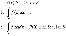
The integrals in properties b and c are multiple intergrals over subsets of Rⁿ, and

dx = dx₁ dx₂ ··· dx_n where x = (x₁, x₂, ..., x_n).

Please do not be intimidated by the multiple integrals. As a practical matter, the evaluation of multiple integrals is more difficult than the evalutation of simple integrals. Conceptually, however, density functions in Rⁿ are no different than density functions in R. Moreover, as we have noted several times before, interesting random experiments almost always involve several random variables (that is, a random vector); seldom do we have a single, isolated random variable.

Property c is particularly important since it implies that the probability distribution of X is completely determined by the density function. Conversely, any function that satisfies properties 1 and 2 is a probability density function, and then property c can be used to define a continuous distribution on S.

Unlike the discrete case, the existence of a density function for a continuous random variable is an assumption that we are making. It is possible for a continuous random variable to not have a density, although such variables are rare in basic probability theory. For an example, however, see the Probability of Winning with Bold Play in the module Red and Black.

Moreover, unlike the discrete case, the density function of a continuous random variable is not unique. Note that the values of f on a finite (or even countable) set of points could be changed to other nonnegative values, and properties a, b, and c would still hold. The key fact is that only integrals of f are important.

The fact that X takes any particular value with probability 0 might seem paradoxical at first, but conceptually it is the same as the fact that an interval of R can have positive length even though it is composed of points each of which has 0 length. Similarly, an region of R² can have positive area even though it is composed of points (or lines) each of which has area 0.

1. Show that if C is a countable subset of S, then

Thus, continuous random variables are in complete contrast with discrete random variables, for which all of the probability mass is concentrated on a discrete set. For a continuous random variable, the probability mass is continuously spread over S. Note also that S itself cannot be countable and in fact must satisfy

If n = 1, S must be a subset of R with positive length; if n = 2, S must be a subset of R² with positive area; if n = 3, S must be a subset of R³ with positive volume.

If we want to, we can always extend f to a density on all of Rⁿ by defining f(x) = 0 for x not in S. This extension sometimes simplifies notation.

Mode

A vector x in S that maximizes the density f is called a mode of the distribution. If there is only one mode, it is sometimes used as a measure of the center of the distribution.

Constructing Densities

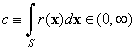
2. Suppose that r is a nonnegative function on S and

Let f(x) = r(x) / c for x in S. Show that the function f is a probability density function on S:

The result in Exercise 2 can be used to construct density functions with desired properties (domain, shape, symmetry, and so on). The constant c is sometimes called the normalizing constant.

3. Let r(x) = x(2 - x) for 0 < x < 2.

1. Find the probability density function f that is proportional to r.
2. Suppose that random variable X has the probability density function f in part a. Find P(1/2 < X < 1).

4. Let r(x) = x^-a for x > 1, where a > 0 is a parameter.

1. Sketch the graph of r.
2. For a > 1, find the probability density function f proportional to r. The resulting distribution is known as the power distribution with parameter a.
3. For 0 < a < 1, show that there is no probability density function proportional to r.
4. Suppose that random variable X has the probability density function f in part b. Find P(1 < X < 2).

5. Let r(x) = 1 / (1 + x²) for x in R.

1. Find the probability density function f that is proportional to r. The resulting distribution is known as the Cauchy distribution.
2. Suppose that random variable X has the probability density function f in part a. Find P(–1 < X < 1).

6. Let r(x, y) = x + y for 0 < x < y < 2.

1. Find the probability density function f that is proportional to r.
2. Suppose that random variable (X, Y) has the probability density function f in part a. Find P(Y > 2X).

7. Let r(x, y) = x²y for 0 < x < 1, 0 < y < 2.

1. Find the probability density function f that is proportional to r.
2. Suppose that random variable (X, Y) has the probability density function f in part a. Find P(X > Y).

Continuous Uniform Distributions

The following problems describe an important class of continuous distributions.

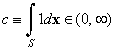
8. Suppose that S is a subset of Rⁿ and that

Let f(x) = 1 / c for x in S. Show that f is a probability density function for a continuous distribution on S:

A random vector X with the density function in Exercise 8 is said to be uniformly distributed over S.

9. In the context of Exercise 8, suppose that n = 1. Show that c is the length of S and that

10. In the context of Exercise 8, suppose that n = 2. Show that c is the area of S and that

11. In the context of Exercise 3, suppose that n = 3. Show that c is the volume of S and that

The uniform distribution on a rectangle in the plane plays a fundamental role in the Buffon's experiments.

Conditional Densities

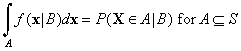
Suppose that X is a continuous random vector taking values in a subset S of Rⁿ. Suppose that the underlying experiment has sample space T, a subset of R^k. The density function of X, of course, is based on the underlying probability measure P for the experiment. This measure could be a conditional probability measure, conditioned on a given event B (a subset of T). The usual notation is

f(x | B), x in S

Note, however, that except for notation, no new concepts are involved. The function above is a continuous density function. That is, it satisfies properties a and b) while property c becomes

All results that hold for densities in general have analogues for conditional densities.

12. Suppose that X has probability density function f(x) = x² / 3 for -1 < x < 2. Find the conditional density of X given X > 0.

13. Suppose that (X, Y) is uniformly distributed on the rectangular region 0 < x < 2, 0 < y < 3. Find the conditional density of (X, Y) given that X < Y.

Distributions