The General Birthday Problem

Java Applet Simulation of the general birthday experiment

Random Variables

Consider again the birthday experiment of distributing k balls randomly into n cells. We record the basic random vector

X = (X₁, X₂, ..., X_k)

where X_i is the number of the cell containing ball i. Mathematically, our modeling assumption is that X is uniformly distributed on the sample space

S = {1, 2, ..., n}^k.

We are interested in two related random variables: the number of empty cells:

and the number of occupied cells:

Note that any cell is either empty or occupied so

U_n,k + V_n,k = n.

Thus, once we have the probability distribution and moments of one variable, we can easily find them for the other variable.

Note also that the simple birthday event that at least one cell has multiple balls can be written as

{V_n,k < k} = {U_n,k > n - k}

The Simulation

In the simulation of the general birthday experiment, the parameters n and k can be varied with scroll bars. When you run the simulation, the basic variables X_i and the cell counts of the occupied cells are shown on each update. The density function and moments of the number of occupied cells V is displayed in the distribution graph and in the distribution table. The value of V is recorded on each update in the record table.

1. In the birthday experiment, set n = 100. Vary k and note the shape of the density graph and its position within the range. With k = 50, run the experiment in single-step mode a few times and observe the outcomes. Now run the experiment 1000 times with an update frequency of 10 and note the apparent convergence of the relative frequency distribution to the true distribution.

The Density Function

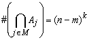
Now let N = {1, 2, ..., n} denote the set of cell indices and for j in N, consider the event that cell j is empty:

Let M be a subset of N with #(M) = m. Using the multiplication principle of combinatorics, it is easy to count the number of ball distributions that leave all the cells indexed by the elements of M empty:

2. Show that

Now the inclusion-exclusion rule of combinatorics can be used to count the number of ball distributions that leave at least one cell empty:

3. Show that

Once we have this, it's simple to count the number of ball distributions that leave no cell empty.

4. Show that

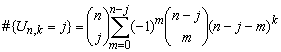
Now we can use a two-step procedure to generate all ball distributions that leave exactly j cells empty: first, choose the j cells that are to be empty. Then distribute the k balls into the remaining cells so that none are empty. Thus, we can use the multiplication principle of combinatorics to count the number of ball distributions that leave exactly j cells empty.

5. Show that

Finally, since our probability distribution P on the sample space is uniform, we can find the density function of the number of empty cells:

6. Show that

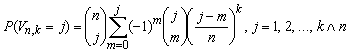
Also, we can easily find the density function of the number of occupied cells:

7. Show that

8. In the birthday experiment, set n = 50. Vary k and note the shape of the density graph and its position within the range. With k = 50 run the experiment in single-step mode a few times and watch the outcomes. Now run the experiment 1000 times with an update frequency of 10 and note the apparent convergence of the relative frequency distribution to the true distribution.

The distribution of the number of empty cells can also be obtained by a recursion argument.

9. Let

Use probability arguments to show that

10. In the birthday experiment, set n = 20. Vary k and note the shape of the density graph and its position within the range. Run the experiment in single-step mode a few times and watch the outcomes. Now run the experiment 1000 times with an update frequency of 10 and note the apparent convergence of the relative frequency distribution to the true distribution.

Moments

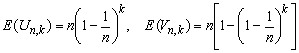
Now we will find the means and variances. The number of empty cells and the number of occupied cells are counting variables and hence can be written as sums of indicator variables. As we have seen in many other models, this representation is frequently the best for computing moments.

Let I_j = 1 if A_j occurs (cell j is empty) and I_j = 0 if A_j does not occur (cell j is occupied).

Note that the number of empty cells can be written as

U_n,k = I₁ + I₂ + ··· + I_n.

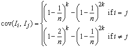
11. Show that

12. Use the results of Exercise 11 to show that

13. Use the result of Exercise 12 to show that

14. Use the results of Exercise 13 and basic properties of variance to show that

15. In the birthday experiment set n = 80. Vary k and note the shape of the density graph and the position and size of the mean-standard deviation bar. With k = 40 run the experiment in single-step mode a few times and watch the outcomes. Now run the experiment 1000 times with an update frequency of 10 and note the apparent convergence of the sample statistics to the distribution parameters.

Cell Counts

16. Let K = (K₁, K₂, ..., K_n) where K_i is the number of balls in cell i for i = 1, 2, ..., n. Show that K has the multinomial distribution:

Ball and Cell Experiments