The Estimate of Pi |
Simulation of Buffon's needle experiment
Suppose that we run Buffon's needle experiment a large number of times. By the very meaning of probability, the proportion of crack crossings should be about the same as the probability of a crack crossing.
More precisely, we will denote the number of crack crossings in the first n runs by Nn. Note that Nn is a random variable for the compound experiment that consists of n replications of the basic needle experiment. Thus, if n is large, we should have
This is Buffon's famous estimate of pi. In the simulation, this estimate is computed on each run and shown numerically in the second table and visually in the bar graph.
![]() 1. Run Buffon's needle experiment with needle
lengths L = 0.3, 0.5, 0.7, and 1. In each case, watch
the estimate of pi as the simulation runs.
1. Run Buffon's needle experiment with needle
lengths L = 0.3, 0.5, 0.7, and 1. In each case, watch
the estimate of pi as the simulation runs.
Let us analyze the estimation problem more carefully. On each run j we have the indicator variable
Ij = 1 if the needle crosses a crack on run j; Ij = 0 otherwise
These indicator variables are independent, and identically distributed, since we are assuming independent replications of the experiment. Thus, the sequence forms a Bernoulli trials process.
![]() 2. Show that the number of crack
crossings in the first n runs of the experiment is
2. Show that the number of crack
crossings in the first n runs of the experiment is
Nn = I1 + I2 + ··· + In.
![]() 3. Use the result of Exercise 1 to
show that the number of crack crossings in the first n runs
has the binomial distribution with parameters n and
3. Use the result of Exercise 1 to
show that the number of crack crossings in the first n runs
has the binomial distribution with parameters n and
![]() 4. Use the result of Exercise 3 to
show that the mean and variance of the number of crack
crossings are
4. Use the result of Exercise 3 to
show that the mean and variance of the number of crack
crossings are
![]() 5. Use the strong law of large numbers to
show that
5. Use the strong law of large numbers to
show that
Thus, we have two basic estimators:
Estimator (1) has several important statistical properties. First, it is unbiased since the expected value of the estimator is the parameter being estimated:
![]() 5. Use Exercise 3 and properties of expected value to
show that
5. Use Exercise 3 and properties of expected value to
show that
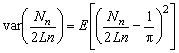
Since this estimator is unbiased, the variance gives the mean square error:
![]() 6. Use Exercise 3 and properties of
variance to show that
6. Use Exercise 3 and properties of
variance to show that
![]() 7. Show that the variance in Exercise
6 is a decreasing function of the needle length L.
7. Show that the variance in Exercise
6 is a decreasing function of the needle length L.
Exercise 7 shows that estimator (1) improves as the needle length increases. Estimator (2) is biased; it tends to overestimate pi:
![]() 8. Use Jensen's inequality to show
that
8. Use Jensen's inequality to show
that
Estimator (2) also tends to improve as the needle length increases. This is not easy to see mathematically. However, you can see it empirically!
![]() 9. Set the update frequency to 100. Run the
simulation 5000 times each with L = 0.3, L = 0.5, L
= 0.7, and L = 1. Note how well the estimator seems to
work in each case.
9. Set the update frequency to 100. Run the
simulation 5000 times each with L = 0.3, L = 0.5, L
= 0.7, and L = 1. Note how well the estimator seems to
work in each case.
Finally, we should note that as a practical matter, Buffon's needle experiment is not a very efficient method of approximating pi. According to Richard Durrett, to estimate pi to four decimal places with L = 1 / 2 would require about 100 million tosses! While it is impractical to test this statement empirically, you can try the following:
![]() 10. Run the simulation with an update frequency
of 100 until the estimates of pi seem to be consistently correct
to two decimal places. Note the number of runs required. Try this
for needle lengths L = 0.3, L = 0.5, L =
0.7, and L = 1 and compare the results.
10. Run the simulation with an update frequency
of 100 until the estimates of pi seem to be consistently correct
to two decimal places. Note the number of runs required. Try this
for needle lengths L = 0.3, L = 0.5, L =
0.7, and L = 1 and compare the results.
Buffon's Experiments |