• General Purpose
• Fit of the Observed Distribution
• Types of Distributions
  • Bernoulli Distribution
  • Beta Distribution
  • Binomial Distribution
  • Cauchy Distribution
  • Chi-square Distribution
  • Exponential Distribution
  • Extreme Value Distribution
  • F Distribution
  • Gamma Distribution
  • Geometric Distribution
  • Gompertz Distribution
  • Laplace Distribution
  • Logistic Distribution
  • Log-normal Distribution
  • Normal Distribution
  • Pareto Distribution
  • Poisson Distribution
  • Rayleigh Distribution
  • Rectangular Distribution
  • Student's t Distribution
  • Weibull Distribution

In some research applications one can formulate hypotheses about the specific distribution of the variable of interest. For example, variables whose values are determined by an infinite number of independent random events will be distributed following the normal distribution: one can think of a person's height as being the result of very many independent factors such as numerous specific genetic predispositions, early childhood diseases, nutrition, etc. (see the animation below for an example of the normal distribution). As a result, height tends to be normally distributed in the U.S. population. On the other hand, if the values of a variable are the result of very rare events, then the variable will be distributed according to the Poisson distribution (sometimes called the distribution of rare events). For example, industrial accidents can be thought of as the result of the intersection of a series of unfortunate (and unlikely) events, and their frequency tends to be distributed according to the Poisson distribution. These and other distributions are described in greater detail in the respective glossary topics.

Another common application where distribution fitting procedures are useful is when one wants to verify the assumption of normality before using some parametric test (see General Purpose of Nonparametric Tests). For example, you may want to use the Kolmogorov-Smirnov test for normality or the Shapiro-Wilks' W test to test for normality.

To index

Fit of the Observed Distribution

For predictive purposes it is often desirable to understand the shape of the underlying distribution of the population. To determine this underlying distribution, it is common to fit the observed distribution to a theoretical distribution by comparing the frequencies observed in the data to the expected frequencies of the theoretical distribution (i.e., a Chi-square goodness of fit test). In addition to this type a test, some software packages also allow you to compute Maximum Likelihood tests and Method of Matching Moments (see Fitting Distributions by Moments in the Process Analysis chapter) tests.

Which Distribution to use. As described above, certain types of variables follow specific distributions. Variables whose values are determined by an infinite number of independent random events will be distributed following the normal distribution, whereas variables whose values are the result of an extremely rare event would follow the Poisson distribution. The major distributions that have been proposed for modeling survival or failure times are the exponential (and linear exponential) distribution, the Weibull distribution of extreme events, and the Gompertz distribution. The section on types of distributions contains a number of distributions generally giving a brief example of what type of data would most commonly follow a specific distribution as well as the probability density functin (pdf) for each distribution.

To index

Types of Distributions

Bernoulli Distribution. This distribution best describes all situations where a "trial" is made resulting in either "success" or "failure," such as when tossing a coin, or when modeling the success or failure of a surgical procedure. The Bernoulli distribution is defined as:

f(x) = p^x *(1-p)^1-x,    for x Î {0,1}

where

p	is the probability that a particular event (e.g., success) will occur.

To index

Beta Distribution. The beta distribution arises from a transformation of the F distribution and is typically used to model the distribution of order statistics. Because the beta distribution is bounded on both sides, it is often used for representing processes with natural lower and upper limits. For examples, refer to Hahn and Shapiro (1967). The beta distribution is defined as:

f(x) = G(n+w)/[G(n)G(w)] * x^n-1*(1-x)^w-1,    for 0 < x < 1, n > 0, w > 0

where

G	is the Gamma function
n, w	are the shape parameters (Shape1 and Shape2, respectively)

The animation above shows the beta distribution as the two shape parameters change.

To index

Binomial Distribution. The binomial distribution is useful for describing distributions of binomial events, such as the number of males and females in a random sample of companies, or the number of defective components in samples of 20 units taken from a production process. The binomial distribution is defined as:

f(x) = [n!/(x!*(n-x)!)]*p^x * q^n-x,    for x = 0,1,2,...,n

where

p	is the probability that the respective event will occur
q	is equal to 1-p
n	is the maximum number of independent trials.

To index

Cauchy Distribution. The Cauchy distribution is interesting for theoretical reasons. Although its mean can be taken as zero, since it is symmetrical about zero, the expectation, variance, higher moments, and moment generating function do not exist. The Cauchy distribution is defined as:

f(x) = 1/(q*p*{1+[(x- h)/ q]²}),    for 0 < q

where

h	is the location parameter (median)
q	is the scale parameter
p	is the constant Pi (3.1415...)

The animation above shows the changing shape of the Cauchy distribution when the location parameter equals 0 and the scale parameter equals 1, 2, 3, and 4.

To index

Chi-square Distribution. The sum of n independent squared random variables, each distributed following the standard normal distribution, is distributed as Chi-square with n degrees of freedom. This distribution is most frequently used in the modeling of random variables (e.g., representing frequencies) in statistical applications. The Chi-square distribution is defined by:

f(x) = {1/[2^n/2* G(n/2)]} * [x^(n/2)-1 * e^-x/2],    for n = 1, 2, ..., 0 < x

where

n	is the degrees of freedom
e	is the base of the natural logarithm, sometimes called Euler's e (2.71...)
G	(gamma) is the Gamma function.

The above animation shows the shape of the Chi-square distribution as the degrees of freedom increase (1, 2, 5, 10, 25 and 50).

To index

Exponential Distribution. If T is the time between occurrences of rare events that happen on the average with a rate l per unit of time, then T is distributed exponentially with parameter l (lambda). Thus, the exponential distribution is frequently used to model the time interval between successive random events. Examples of variables distributed in this manner would be the gap length between cars crossing an intersection, life-times of electronic devices, or arrivals of customers at the check-out counter in a grocery store. The exponential distribution function is defined as:

f(x) = l*e^-lx    for 0 £ x < ¥, l > 0

where

l	is an exponential function parameter (an alternative parameterization is scale parameter b=1/l)
e	is the base of the natural logarithm, sometimes called Euler's e (2.71...)

To index

Extreme Value. The extreme value distribution is often used to model extreme events, such as the size of floods, gust velocities encountered by airplanes, maxima of stock marked indices over a given year, etc.; it is also often used in reliability testing, for example in order to represent the distribution of failure times for electric circuits (see Hahn and Shapiro, 1967). The extreme value (Type I) distribution has the probability density function:

f(x) = 1/b * e^[-(x-a)/b] * e^{-e^[-(x-a)/b]},    for -¥ < x < ¥, b > 0

where

a	is the location parameter
b	is the scale parameter
e	is the base of the natural logarithm, sometimes called Euler's e (2.71...)

To index

F Distribution. Snedecor's F distribution is most commonly used in tests of variance (e.g., ANOVA). The ratio of two chi-squares divided by their respective degrees of freedom is said to follow an F distribution. The F distribution (for x > 0) has the probability density function (for n = 1, 2, ...; w = 1, 2, ...):

f(x) = [G{(n+w)/2}]/[G(n/2)G(w/2)] * (n/w)^(n/2) * x^[(n/2)-1] * {1+[(n/w)*x]}^[-(n+w)/2],    for 0 £ x < ¥ n=1,2,..., w=1,2,...

where

n, w	are the shape parameters, degrees of freedom
G	is the Gamma function

The animation above shows various tail areas (p-values) for an F distribution with both degrees of freedom equal to 10.

To index

Gamma Distribution. The probability density function of the exponential distribution has a mode of zero. In many instances, it is known a priori that the mode of the distribution of a particular random variable of interest is not equal to zero (e.g., when modeling the distribution of the life-times of a product such as an electric light bulb, or the serving time taken at a ticket booth at a baseball game). In those cases, the gamma distribution is more appropriate for describing the underlying distribution. The gamma distribution is defined as:

f(x) = {1/[bG(c)]}*[x/b]^c-1*e^-x/b    for 0 £ x, c > 0

where

G	is the Gamma function
c	is the Shape parameter
b	is the Scale parameter.
e	is the base of the natural logarithm, sometimes called Euler's e (2.71...)

The animation above shows the gamma distribution as the shape parameter changes from 1 to 6.

To index

Geometric Distribution. If independent Bernoulli trials are made until a "success" occurs, then the total number of trials required is a geometric random variable. The geometric distribution is defined as:

f(x) = p*(1-p)^x,    for x = 1,2,...

where

p	is the probability that a particular event (e.g., success) will occur.

To index

Gompertz Distribution. The Gompertz distribution is a theoretical distribution of survival times. Gompertz (1825) proposed a probability model for human mortality, based on the assumption that the "average exhaustion of a man's power to avoid death to be such that at the end of equal infinetely small intervals of time he lost equal portions of his remaining power to oppose destruction which he had at the commencement of these intervals" (Johnson, Kotz, Blakrishnan, 1995, p. 25). The resultant hazard function:

r(x)=Bc^x,    for x £ 0, B > 0, c £ 1

is often used in survival analysis. See Johnson, Kotz, Blakrishnan (1995) for additional details.

To index

Laplace Distribution. For interesting mathematical applications of the Laplace distribution see Johnson and Kotz (1995). The Laplace (or Double Exponential) distribution is defined as:

f(x) = 1/(2b) * e^[-(|x-a|/b)],    for -¥ < x < ¥

where

a	is the location parameter (mean)
b	is the scale parameter
e	is the base of the natural logarithm, sometimes called Euler's e (2.71...)

The graphic above shows the changing shape of the Laplace distribution when the location parameter equals 0 and the scale parameter equals 1, 2, 3, and 4.

To index

Logistic Distribution. The logistic distribution is used to model binary responses (e.g., Gender) and is commonly used in logistic regression. The logistic distribution is defined as:

f(x) = (1/b) * e^[-(x-a)/b] * {1+e^{[-(x-a)/b]}^-2},    for -¥ < x < ¥, 0 < b

where

a	is the location parameter (mean)
b	is the scale parameter
e	is the base of the natural logarithm, sometimes called Euler's e (2.71...)

The graphic above shows the changing shape of the logistic distribution when the location parameter equals 0 and the scale parameter equals 1, 2, and 3.

To index

Log-normal Distribution. The log-normal distribution is often used in simulations of variables such as personal incomes, age at first marriage, or tolerance to poison in animals. In general, if x is a sample from a normal distribution, then y = e^x is a sample from a log-normal distribution. Thus, the log-normal distribution is defined as:

f(x) = 1/[xs(2)^1/2] * e^{-[log(x)-m]**2/2s**2},    for 0 < x < ¥, m > 0, s > 0

where

m	is the scale parameter
s	is the shape parameter
e	is the base of the natural logarithm, sometimes called Euler's e (2.71...)

The animation above shows the log-normal distribution with mu equal to 0 for sigma equals .10, .30, .50, .70, and .90.

To index

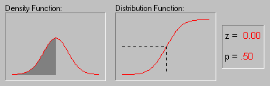
Normal Distribution. The normal distribution (the "bell-shaped curve" which is symmetrical about the mean) is a theoretical function commonly used in inferential statistics as an approximation to sampling distributions (see also Elementary Concepts). In general, the normal distribution provides a good model for a random variable, when:

1. There is a strong tendency for the variable to take a central value;
2. Positive and negative deviations from this central value are equally likely;
3. The frequency of deviations falls off rapidly as the deviations become larger.

f(x) = 1/[(2*p)^1/2*s] * e**{-1/2*[(x-m)/s]² },    for -¥ < x < ¥

where

m	is the mean
s	is the standard deviation
e	is the base of the natural logarithm, sometimes called Euler's e (2.71...)
p	is the constant Pi (3.14...)

The animation above shows several tail areas of the standard normal distribution (i.e., the normal distribution with a mean of 0 and a standard deviation of 1). The standard normal distribution is often used in hypothesis testing.

To index

Pareto Distribution. The Pareto distribution is commonly used in monitoring production processes (see Quality Control and Process Analysis). For example, a machine which produces copper wire will occasionally generate a flaw at some point along the wire. The Pareto distribution can be used to model the length of wire between successive flaws. The standard Pareto distribution is defined as:

f(x) = c/x^c+1,    for 1 £ x, c < 0

where

c	is the shape parameter

The animation above shows the Pareto distribution for the shape parameter equal to 1, 2, 3, 4, and 5.

To index

Poisson Distribution. The Poisson distribution is also sometimes referred to as the distribution of rare events. Examples of Poisson distributed variables are number of accidents per person, number of sweepstakes won per person, or the number of catastrophic defects found in a production process. It is defined as:

f(x) = (l^x*e^-l)/x!,    for x = 0,1,2,..., 0 < l

where

l	(lambda) is the expected value of x (the mean)
e	is the base of the natural logarithm, sometimes called Euler's e (2.71...)

To index

Rayleigh Distribution. If two independent variables y₁ and y₂ are independent from each other and normally distributed with equal variance, then the variable x = Ö(y₁²+ y₂²) will follow the Rayleigh distribution. Thus, an example (and appropriate metaphor) for such a variable would be the distance of darts from the target in a dart-throwing game, where the errors in the two dimensions of the target plane are independent and normally distributed. The Rayleigh distribution is defined as:

f(x) = x/b² * e^[-(x²/2b²)],    for 0 £ x < ¥, b > 0

where

b	is the scale parameter
e	is the base of the natural logarithm, sometimes called Euler's e (2.71...)

The graphic above shows the changing shape of the Rayleigh distribution when the scale parameter equals 1, 2, and 3.

To index

Rectangular Distribution. The rectangular distribution is useful for describing random variables with a constant probability density over the defined range a<b.

f(x) = 1/(b-a),    for a<x<b
       = 0 ,           elswhere

where

a<b	are constants.

To index

Student's t Distribution. The student's t distribution is symmetric about zero, and its general shape is similar to that of the standard normal distribution. It is most commonly used in testing hypothesis about the mean of a particular population. The student's t distribution is defined as (for n = 1, 2, . . .):

f(x) = G[(n+1)/2] / G(n/2) * (n*p)^-1/2 * [1 + (x²/n)^-(n+1)/2

where

n	is the shape parameter, degrees of freedom
G	is the Gamma function
p	is the constant Pi (3.14 . . .)

The shape of the student's t distribution is determined by the degrees of freedom. As shown in the animation above, its shape changes as the degrees of freedom increase.

To index

Weibull Distribution. As described earlier, the exponential distribution is often used as a model of time-to-failure measurements, when the failure (hazard) rate is constant over time. When the failure probability varies over time, then the Weibull distribution is appropriate. Thus, the Weibull distribution is often used in reliability testing (e.g., of electronic relays, ball bearings, etc.; see Hahn and Shapiro, 1967). The Weibull distribution is defined as:

f(x) = c/b*(x/b)^(c-1) * e^{[-(x/b)^c]},    for 0 £ x < ¥, b > 0, c > 0

where

b	is the scale parameter
c	is the shape parameter
e	is the base of the natural logarithm, sometimes called Euler's e (2.71...)

The animation above shows the Weibull distribution as the shape parameter increases (.5, 1, 2, 3, 4, 5, and 10).

To index