Introductory Statistics: Concepts, Models, and Applications
David W. Stockburger
Hypothesis tests may be performed on contingency tables in order to decide whether or not effects are present. Effects in a contingency table are defined as relationships between the row and column variables; that is, are the levels of the row variable diferentially distributed over levels of the column variables. Significance in this hypothesis test means that interpretation of the cell frequencies is warranted. Non-significance means that any differences in cell frequencies could be explained by chance.
Hypothesis tests on contingency tables are based on a statistic called Chi-square. In this chapter contingency tables will first be reviewed, followed by a discussion of the Chi-squared statistic. The sampling distribution of the Chi-squared statistic will then be presented, preceded by a discussion of the hypothesis test. A complete computational example will conclude the chapter.
Frequency tables of two variables presented simultaneously are called contingency tables. Contingency tables are constructed by listing all the levels of one variable as rows in a table and the levels of the other variables as columns, then finding the joint or cell frequency for each cell. The cell frequencies are then summed across both rows and columns. The sums are placed in the margins, the values of which are called marginal frequencies. The lower right hand corner value contains the sum of either the row or column marginal frequencies, which both must be equal to N.
For example, suppose that a researcher studied the relationship between having the AIDS Syndrome and sexual preference of individuals. The study resulted in the following data for thirty male subjects:
AIDS
|
NY |
Y |
N |
N |
N |
Y |
N |
N |
N |
Y |
N |
N |
N |
Y |
N |
N |
N |
N |
N |
N |
N |
Y |
N |
Y |
Y |
N |
Y |
N |
Y |
N |
|
M |
B |
F |
F |
B |
F |
F |
F |
M |
F |
F |
F |
F |
B |
F |
F |
B |
F |
M |
F |
F |
M |
F |
B |
M |
F |
M |
F |
M |
F |
SEXPREF
with Y = "yes" and N = "no" for AIDS and F = "female", M = "male" and B = "both" for SEXPREF.
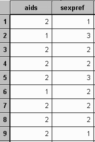
The data file, with coding AIDS (1="Yes" and 2="No") and SEXPREF (1="Males", 2="Females, and 3="Both"), would appear as follows:

A contingency table and chi-square hypothesis test of independence could be generated using the following commands:
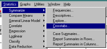
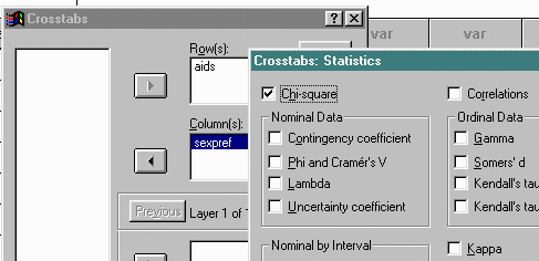
The resulting output tables are presented below:
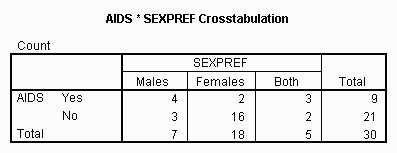
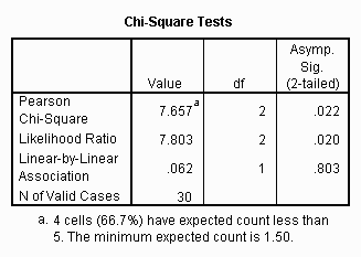
The fact that the Pearson chi-square value under "Asymp. Sig" is 0.022 and less than .05 indicates that the rows and columns of the contingency are independent. In general this means that it is worthwhile to interpret the cells in the contingency table. In this particular case it means that the AIDS Syndrome is not distributed similarly across the different levels of sexual preference. In other words, males who prefer other males or both males and females are more likely to have the syndrome than males who prefer females.
The procedure used to test the significance of contingency tables is similar to all other hypothesis tests. That is, a statistic is computed and then compared to a model of what the world would look like if the experiment was repeated an infinite number of times when there were no effects. In this case the statistic computed is called the chi-square statistic. This statistic will be discussed first, followed by a discussion of its theoretical distribution. Finding critical values of chi-square and its interpretation will conclude the chapter.
The first step in computing the Chi-squared statistic is the computation of the contingency table. The preceding table is reproduced below:
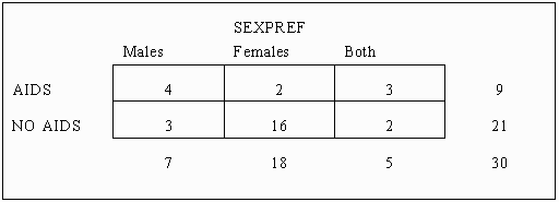
The next step in computing the Chi-squared statistic is the computation of the expected cell frequency for each cell. This is accomplished by multiplying the marginal frequencies for the row and column (row and column totals) of the desired cell and then dividing by the total number of observations. The formula for computation can be represented as follows:
Expected Cell Frequency = (Row Total * Column Total) / N
For example, computation of the expected cell frequency for Males with AIDS would proceed as follows:
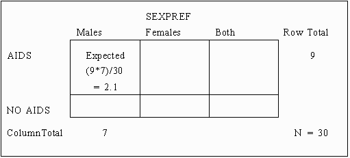
Expected Cell Frequency = (Row Total * Column Total) / N
= ( 9 * 7 ) / 30 = 2.1
Using the same procedure to compute all the expected cell frequencies results in the following table:
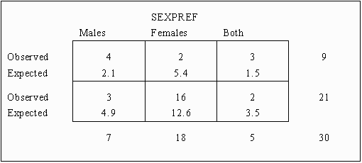
The next step is to subtract the expected cell frequency from the observed cell frequency for each cell. This value gives the amount of deviation or error for each cell. Adding these to the preceding table results in the following:
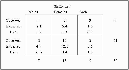
Note that the sum of the expected row total is the same as the sum of the observed row totals; the same holds true for the column totals. Note also that the sum of the Observed - Expected for both the rows and columns equals zero.
Following this, the difference computed in the last step is squared, resulting in the following table:
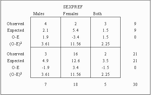
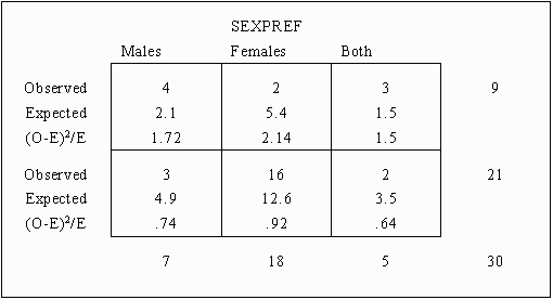
Each of the squared differences is then divided by the expected cell frequency for each cell, resulting in the following table:

The chi-square statistic is computed by summing the last row of each cell in the preceding table, the formula being represented by:
![]()
This computation for the example table would result in the following:
![]() = 1.72 + 2.14 + 1.50 + .74 + .92 + .64 = 7.66
= 1.72 + 2.14 + 1.50 + .74 + .92 + .64 = 7.66
Note that this value is within rounding error of the value for Chi-square computed by the computer in an earlier section of this chapter.
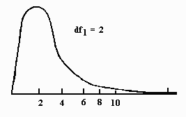
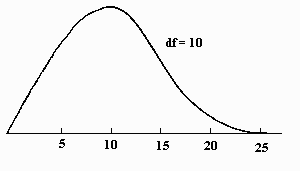
The distribution of the chi-square statistic may be specified given the preceding experiment were conducted an infinite number of times and the effects were not real. The resulting distribution is called the chi-square distribution. The chi-square distribution is characterized by a parameter called the degrees of freedom (df) which determines the shape of the distribution. Two chi-square distributions are presented below for two different values of the degrees of freedom parameter.
The degrees of freedom in the example chi-square is computed by multiplying one minus the number of rows, times one minus the number of columns. The procedure is represented below:
df = ( #Rows - 1 ) * ( #Columns -1)
In the example problem the degrees of freedom is equal to ( 2 - 1 ) * ( 3 - 1 ) = 1 * 2 = 2.
The critical values for almost any Chi-square distribution can be estimated from the Chi-square program included with this book. The use of this program is illustrated below for a distribution with two degrees of freedom.
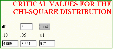
A model of what the distribution of Chi-square statistics would look like given there really was no relationship between sexual preference and whether or not an individual has the AIDS Syndrome is described by the first example Chi-square distribution. The following illustration includes the critical values.
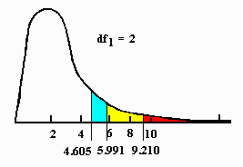
Note that the area falling above a value of 7.66 is about midway between the critical value for Chi-square when alpha is .05 and .01. The SPSS computer output gives an exact "Sig." level of .022. This makes it unnecessary to look up the critical value of Chi-square because the computer has already done so. All that is necessary is to compare the resulting "Sig" level with alpha. If this value is less than alpha, the hypothesis test is significant. If it is greater than alpha, then the null hypothesis of independence must be retained.
The observed value, which is computed using the procedure outlined previously in this chapter, is compared with the critical value found using the chi-square program. If the observed value is greater than the expected value, the model of no effects is rejected, as is the assumption of no effects. The table is said to be significant and an interpretation of cell frequencies is warranted. This is the case in the example problem.
The interpretation of the cell frequencies may be guided by the amount each cell contributes to the chi-squared statistic, as seen in the (O-E)2/E value. In general, the larger the difference between the observed and expected values, the greater this value. In the example data, it can be seen that the homosexual males had a greater incidence of Aids (Observed = 4, Expected = 2.1) than would be expected by chance alone, while heterosexual had a lesser incidence (Observed = 2, Expected = 5.4). This sort of evidence could direct the search for the causes of Aids.
If the value of the observed chi-square statistic is less than the expected value, then the model of no effects cannot be rejected and the table is not significant. It can be said that no effects were discovered. In this case an interpretation of the cell frequencies is not required, because the values could have been obtained by chance alone.
The chi-square test of significance is useful as a tool to determine whether or not it is worth the researcher's effort to interpret a contingency table. A significant result of this test means that the cells of a contingency table should be interpreted. A non-significant test means that no effects were discovered and chance could explain the observed differences in the cells. In this case, an interpretation of the cell frequencies is not useful.