Introductory Statistics: Concepts, Models, and Applications
David W. Stockburger
Suppose a researcher has performed a study on the effectiveness of various methods of individual therapy. The methods used were: Reality Therapy, Behavior Therapy, Psychoanalysis, Gestalt Therapy, and, of course, a control group. Twenty patients were randomly assigned to each group. At the conclusion of the study, changes in self-concept were found for each patient. The purpose of the study was to determine if one method was more effective than the other methods.
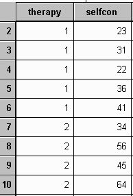
At the conclusion of the experiment the researcher creates a data file in SPSS in the following manner:

The researcher wishes to compare the means of the groups to decide about the effectiveness of the therapy.
One method of performing this analysis is by doing all possible t-tests, called multiple t-tests. That is, Reality Therapy is first compared with Behavior Therapy, then Psychoanalysis, then Gestalt Therapy, and then the Control Group. Behavior Therapy is then individually compared with the last three groups, and so on. Using this procedure there would be ten different t-tests performed. Therein lies the difficulty with multiple t-tests.
First, because the number of t-tests increases geometrically as a function of the number of groups, analysis becomes cognitively difficult somewhere in the neighborhood of seven different tests. An analysis of variance organizes and directs the analysis, allowing easier interpretation of results.
Second, by doing a greater number of analyses, the probability of committing at least one type I error somewhere in the analysis greatly increases. The probability of committing at least one type I error in an analysis is called the experiment-wise error rate. The researcher may desire to perform a fewer number of hypothesis tests in order to reduce the experiment-wise error rate. The ANOVA procedure performs this function.
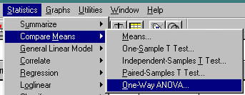
In this case, the correct analysis in SPSS is a one-way ANOVA. The one-way ANOVA procedure is selected in the following manner.

The results of the optional "Descriptive" button of the above procedure are a table of means and standard deviations.

The results of the ANOVA are presented in an ANOVA table. This table contains columns labeled "Source", "SS or Sum of Squares", "df - for degrees of freedom", "MS - for mean square", "F or F-ratio", and "p, prob, probability, sig., or sig. of F". The only columns that are critical for interpretation are the first and the last! The others are used mainly for intermediate computational purposes. An example of an ANOVA table appears below:

The row labelled "Between Groups" , having a probability value associated with it, is the only one of any great importance at this time. The other rows are used mainly for computational purposes. The researcher would most probably first look at the value ".000" located under the "Sig." column.
Of all the information presented in the ANOVA table, the major interest of the researcher will most likely be focused on the value located in the "Sig." column. If the number (or numbers) found in this column is (are) less than the critical value (![]() ) set by the experimenter, then the effect is said to be significant. Since this value is usually set at .05, any value less than this will result in significant effects, while any value greater than this value will result in nonsignificant effects.
) set by the experimenter, then the effect is said to be significant. Since this value is usually set at .05, any value less than this will result in significant effects, while any value greater than this value will result in nonsignificant effects.
If the effects are found to be significant using the above procedure, it implies that the means differ more than would be expected by chance alone. In terms of the above experiment, it would mean that the treatments were not equally effective. This table does not tell the researcher anything about what the effects were, just that there most likely were real effects.
If the effects are found to be nonsignificant, then the differences between the means are not great enough to allow the researcher to say that they are different. In that case, no further interpretation is attempted.
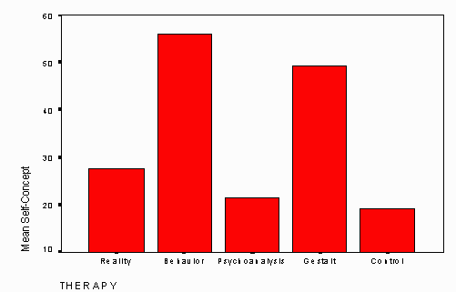
When the effects are significant, the means must then be examined in order to determine the nature of the effects. There are procedures called "post-hoc tests" to assist the researcher in this task, but often the analysis is fairly evident simply by looking at the size of the various means. For example, in the preceding analysis, Gestalt and Behavior Therapy were the most effective in terms of mean improvement.
In the case of significant effects, a graphical presentation of the means can sometimes assist in analysis. For example, in the preceding analysis, the graph of mean values would appear as follows:
In order to explain why the above procedure may be used to simultaneously analyze a number of means, the following presents the theory on ANOVA, in relation to the hypothesis testing approach discussed in earlier chapters.
First, a review of the sampling distribution is necessary. If you have difficulty with this summary, please go back and read the more detailed chapter on the sampling distribution.
A sample is a finite number (N) of scores. Sample statistics are numbers which describe the sample. Example statistics are the mean (![]() ), mode (Mo), median (Md), and standard deviation (sX).
), mode (Mo), median (Md), and standard deviation (sX).
Probability models exist in a theoretical world where complete information is unavailable. As such, they can never be known except in the mind of the mathematical statistician. If an infinite number of infinitely precise scores were taken, the resulting distribution would be a probability model of the population. Population models are characterized by parameters. Two common parameters are ![]() and
and ![]() .
.
Sample statistics are used as estimators of the corresponding parameters in the population model. For example, the mean and standard deviation of the sample are used as estimates of the corresponding population parameters ![]() and
and ![]() .
.
The sampling distribution is a distribution of a sample statistic. It is a model of a distribution of scores, like the population distribution, except that the scores are not raw scores, but statistics. It is a thought experiment; "What would the world be like if a person repeatedly took samples of size N from the population distribution and computed a particular statistic each time?" The resulting distribution of statistics is called the sampling distribution of that statistic.
The sampling distribution of the mean is a special case of a sampling distribution. It is a distribution of sample means, described with the parameters ![]() and
and ![]() . These parameters are closely related to the parameters of the population distribution, the relationship being described by the CENTRAL LIMIT THEOREM. The CENTRAL LIMIT THEOREM essentially states that the mean of the sampling distribution of the mean (
. These parameters are closely related to the parameters of the population distribution, the relationship being described by the CENTRAL LIMIT THEOREM. The CENTRAL LIMIT THEOREM essentially states that the mean of the sampling distribution of the mean (![]() ) equals the mean of the population (
) equals the mean of the population (![]() ), and that the standard error of the mean (
), and that the standard error of the mean (![]() ) equals the standard deviation of the population (
) equals the standard deviation of the population (![]() ) divided by the square root of N. These relationships may be summarized as follows:
) divided by the square root of N. These relationships may be summarized as follows:

When the data have been collected from more than one sample, there exists two independent methods of estimating the population parameter ![]() , called respectively the between and the within method. The collected data are usually first described with sample statistics, as demonstrated in the following example:
, called respectively the between and the within method. The collected data are usually first described with sample statistics, as demonstrated in the following example:
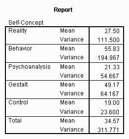
Since each of the sample variances may be considered an independent estimate of the parameter ![]() , finding the mean of the variances provides a method of combining the separate estimates of
, finding the mean of the variances provides a method of combining the separate estimates of ![]() into a single value. The resulting statistic is called the MEAN SQUARES WITHIN, often represented by MSW. It is called the within method because it computes the estimate by combining the variances within each sample. In the above example, the Mean Squares Within would be equal to 89.78.
into a single value. The resulting statistic is called the MEAN SQUARES WITHIN, often represented by MSW. It is called the within method because it computes the estimate by combining the variances within each sample. In the above example, the Mean Squares Within would be equal to 89.78.
![]()
The parameter ![]() may also be estimated by comparing the means of the different samples, but the logic is slightly less straightforward and employs both the concept of the sampling distribution and the Central Limit Theorem.
may also be estimated by comparing the means of the different samples, but the logic is slightly less straightforward and employs both the concept of the sampling distribution and the Central Limit Theorem.
First, the standard error of the mean squared (![]() ) is the population variance of a distribution of sample means. In real life, in the situation where there is more than one sample, the variance of the sample means may be used as an estimate of the standard error of the mean squared (
) is the population variance of a distribution of sample means. In real life, in the situation where there is more than one sample, the variance of the sample means may be used as an estimate of the standard error of the mean squared (![]() ). This is analogous to the situation where the variance of the sample (s2) is used as an estimate of
). This is analogous to the situation where the variance of the sample (s2) is used as an estimate of ![]() .
.
In this case the Sampling Distribution consists of an infinite number of means and the real life data consists of A (in this case 5) means. The computed statistic is thus an estimate of the theoretical parameter.
The relationship expressed in the Central Limit Theorem may now be used to obtain an estimate of ![]() .
.

Thus the variance of the population may be found by multiplying the standard error of the mean squared (![]() ) by N, the size of each sample.
) by N, the size of each sample.
Since the variance of the means, ![]() , is an estimate of the standard error of the mean squared,
, is an estimate of the standard error of the mean squared, ![]() , the variance of the population,
, the variance of the population, ![]() , may be estimated by multiplying the size of each sample, N, by the variance of the sample means. This value is called the Mean Squares Between and is often symbolized by MSB. The computational procedure for MSB is presented below:
, may be estimated by multiplying the size of each sample, N, by the variance of the sample means. This value is called the Mean Squares Between and is often symbolized by MSB. The computational procedure for MSB is presented below:
![]()
The expressed value is called the Mean Squares Between, because it uses the variance between the sample means to compute the estimate. Using the above procedure on the example data yields:

At this point it has been established that there are two methods of estimating ![]() , Mean Squares Within and Mean Squares Between. It could also be demonstrated that these estimates are independent. Because of this independence, when both mean squares are computed using the same data set, different estimates will result. For example, in the presented data MSW=89.78 while MSB=1699.28. This difference provides the theoretical background for the F-ratio and ANOVA.
, Mean Squares Within and Mean Squares Between. It could also be demonstrated that these estimates are independent. Because of this independence, when both mean squares are computed using the same data set, different estimates will result. For example, in the presented data MSW=89.78 while MSB=1699.28. This difference provides the theoretical background for the F-ratio and ANOVA.
A new statistic, called the F-ratio is computed by dividing the MSB by MSW. This is illustrated below:

Using the example data described earlier the computed F-ratio becomes:

The F-ratio can be thought of as a measure of how different the means are relative to the variability within each sample. The larger this value, the greater the likelihood that the differences between the means are due to something other than chance alone, namely real effects. How big this F-ratio needs to be in order to make a decision about the reality of effects is the next topic of discussion.
If the difference between the means is due only to chance, that is, there are no real effects, then the expected value of the F-ratio would be one (1.00). This is true because both the numerator and the denominator of the F-ratio are estimates of the same parameter, ![]() . Seldom will the F-ratio be exactly equal to 1.00, however, because the numerator and the denominator are estimates rather than exact values. Therefore, when there are no effects the F-ratio will sometimes be greater than one, and other times less than one.
. Seldom will the F-ratio be exactly equal to 1.00, however, because the numerator and the denominator are estimates rather than exact values. Therefore, when there are no effects the F-ratio will sometimes be greater than one, and other times less than one.
To review, the basic procedure used in hypothesis testing is that a model is created in which the experiment is repeated an infinite number of times when there are no effects. A sampling distribution of a statistic is used as the model of what the world would look like if there were no effects. The results of the experiment, a statistic, is compared with what would be expected given the model of no effects was true. If the computed statistic is unlikely given the model, then the model is rejected, along with the hypothesis that there were no effects.
In an ANOVA, the F-ratio is the statistic used to test the hypothesis that the effects are real: in other words, that the means are significantly different from one another. Before the details of the hypothesis test may be presented, the sampling distribution of the F-ratio must be discussed.
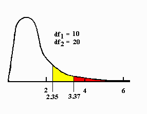
If the experiment were repeated an infinite number of times, each time computing the F-ratio, and there were no effects, the resulting distribution could be described by the F-distribution. The F-distribution is a theoretical probability distribution characterized by two parameters, df1 and df2, both of which affect the shape of the distribution. Since the F-ratio must always be positive, the F-distribution is non-symmetrical, skewed in the positive direction.
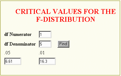
The F-ratio which cuts off various proportions of the distributions may be computed for different values of df1 and df2. These F-ratios are called Fcrit values and may be found by entering the appropriate values for degrees of freedom in the F-distribution program.
Two examples of an F-distribution are presented below; the first with df1=10 and df2=25, and the second with df1=1 and df2=5. Preceding each distribution is an example of the use of the F-distribution to find Fcrit

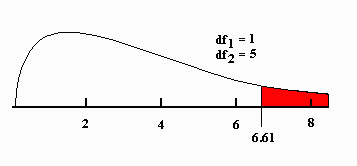
The F-distribution has a special relationship to the t-distribution described earlier. When df1=1, the F-distribution is equal to the t-distribution squared (F=t2). Thus the t-test and the ANOVA will always return the same decision when there are two groups. That is, the t-test is a special case of ANOVA.
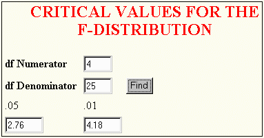
Theoretically, when there are no real effects, the F-distribution is an accurate model of the distribution of F-ratios. The F-distribution will have the parameters df1=A-1 (where A-1 is the number of different groups minus one) and df2=A(N-1), where A is the number of groups and N is the number in each group. In this case, an assumption is made that sample size is equal for each group. For example, if five groups of six subjects each were run in an experiment, and there were no effects, the F-ratios would be distributed with df1= A-1 = 5-1 = 4 and df2= A(N-1) = 5(6-1)=5*5=25. A visual representation of the preceding appears as follows:
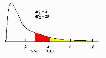
When there are real effects, that is, the means of the groups are different due to something other than chance; the F-distribution no longer describes the distribution of F-ratios. In almost all cases, the observed F-ratio will be larger than would be expected when there were no effects. The rationale for this situation is presented below.
First, an assumption is made that any effects are an additive transformation of the score. That is, the scores for each subject in each group can be modeled as a constant ( aa - the effect) plus error (eae). The scores appear as follows:
![]()
Xae is the score for Subject e in group a, aa is the size of the treatment effect, and eae is the size of the error. The eae, or error, is different for each subject, while aa is constant within a given group.
As described in the chapter on transformations, an additive transformation changes the mean, but not the standard deviation or the variance. Because the variance of each group is not changed by the nature of the effects, the Mean Square Within, as the mean of the variances, is not affected. The Mean Square Between, as N time the variance of the means, will in most cases become larger because the variance of the means will most likely become larger.
Imagine three individuals taking a test. An instructor first finds the variance of the three scores. He or she then adds five points to one random individual and subtracts five from another random individual. In most cases the variance of the three test score will increase, although it is possible that the variance could decrease if the points were added to the individual with the lowest score and subtracted from the individual with the highest score. If the constant added and subtracted was 30 rather than 5, then the variance would almost certainly be increased. Thus, the greater the size of the constant, the greater the likelihood of a larger increase in the variance.
With respect to the sampling distribution, the model differs depending upon whether or not there are effects. The difference is presented below:
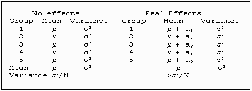
Since the MSB usually increases and MSW remains the same, the F-ratio (F=MSB/MSW) will most likely increase. Thus, if there are real effects, then the F-ratio obtained from the experiment will most likely be larger than the critical level from the F-distribution. The greater the size of the effects, the larger the obtained F-ratio is likely to become.
Thus, when there are no effects, the obtained F-ratio will be distributed as an F-distribution that may be specified. If effects exist, the obtained F-ratio will most likely become larger. By comparing the obtained F-ratio with that predicted by the model of no effects, a hypothesis test may be performed to decide on the reality of effects. If the obtained F-ratio is greater than the critical F-ratio, the decision will be that the effects are real. If not, then no decision about the reality of effects can be made.
When the number of groups (A) equals two (2), an ANOVA and t-test will give similar results, with t2crit = Fcrit and t2obs = Fobs. This equality is demonstrated in the example below:
Given the following numbers for two groups:
|
Group |
|
|
|||||||||
|
1 |
12 |
23 |
14 |
21 |
19 |
23 |
26 |
11 |
16 |
18.33 |
28.50 |
|
2 |
10 |
17 |
20 |
14 |
23 |
11 |
14 |
15 |
19 |
15.89 |
18.11 |
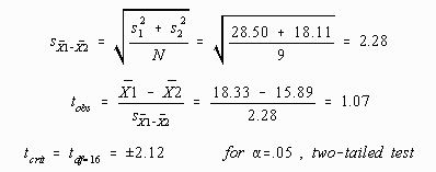
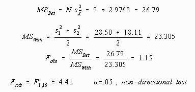

The differences between the predicted and observed results can be attributed to rounding error (close enough for government work).
Because the t-test is a special case of the ANOVA and will always yield similar results, most researchers perform the ANOVA because the technique is much more powerful in complex experimental designs.
Given the following data for five groups, perform an ANOVA:


Since the Fcrit = 2.76 is greater than the Fobs= 1.297, the means are not significantly different and no effects are said to be discovered. Because SPSS output includes "Sig.", all that is necessary is to compare this value (.298) with alpha, in this case .05. Since the "Sig." level is greater than alpha, the results are not significant.
Given the following data for five groups, perform an ANOVA. Note that the numbers are similar to the previous example except that three has been added to Group 1, six to Group 2, nine to Group 3, twelve to Group 4, and fifteen to Group 5. This is equivalent to adding effects (aa) to the scores. Note that the means change, but the variances do not.


In this case, the FOBS = 2.79 is greater than FCRIT= 2.76; thus the means are significantly different and we decide that the effects are real. Note that the "Sig." value is less than .05. It is not much less, however. If the alpha level had been set at .01, or even .045, the results of the hypothesis test would not be significant. In classical hypothesis testing, however, there is no such thing as "close"; the results are either significant or not significant. In practice, however, researchers will often report the actual "Sig." value and let the reader set his or her own significance level. When this is done the distinction between Bayesian and Classical Hypothesis Testing approaches becomes somewhat blurred. Personally I feel that anything that gives the reader more information about your data without a great deal of cognitive effort is valuable and should be done. The reader should be aware that many other statisticians do not agree with me and would oppose the reporting of exact significance levels.