A nested t-test is the appropriate hypothesis test when there are two groups and different subjects are used in the treatment groups. Two illustrations of nested t-tests will be presented in this chapter, one detailing the logic underlying the analysis and one illustrating the manner in which the analysis will be performed in practice.

ANALYSIS AND LOGIC UNDERLYING NESTED DESIGNS

In a comparison of the finger-tapping speed of males and females the following data was collected:

The design is necessarily nested because each subject has only one score and appears in a single treatment condition. Through the marvels of modern medicine it might be possible to treat sex as a crossed design, but finding subjects might be somewhat difficult. The next step is to find the mean and variance of the two groups:

The critical statistic is the difference between the two means . In the example, it is noted that females, on the average, tapped faster than males. A difference of 43.33 - 57.33 or -14.00 was observed between the two means. The question addressed by the hypothesis test is whether this difference is large enough to consider the effect to be due to a real difference between males and females, rather than a chance happening (the sample of females just happened to be faster than the sample of males).

The analysis proceeds in a manner similar to all hypothesis tests. An assumption is made that there is no difference in the tapping speed of males and females. The experiment is then carried out an infinite number of times, each time finding the difference between means, creating a model of the world when the Null Hypothesis is true. The difference between the means that was obtained is compared to the difference that would be expected on the basis of the model of no effects. If the difference that was found is unlikely given the model, the model of no effects is rejected and the difference is said to be significant.

In the case of a nested design, the sampling distribution is the difference between means. The sampling distribution consists of an infinite number of differences between means.

This sampling distribution of this statistic is characterized by the parameters and . In the case of , if the null hypothesis is true, then the mean of the sampling distribution would be equal to zero (0). The value of is not known, but may be estimated. In each of the following formulas, the assumption is made that the variances of the population values of for each group are similar.

The computational formula for the estimate of the standard error of the difference between means is the following:

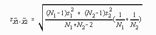
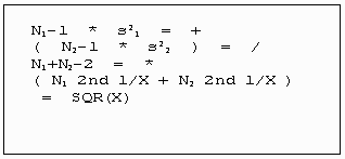
The procedure for finding the value of this statistic using a statistical calculator with parentheses is as follows:

If each group has the same number of scores then the preceding formula may be simplified:

if N1 = N2 = N then

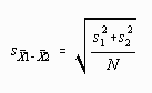
Because the example problem has different numbers in each group, the longer formula must be used. Computation proceeds as follows:

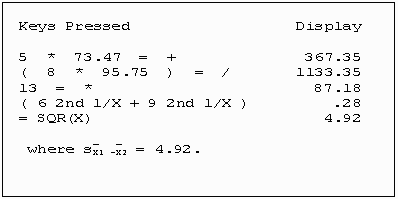
The sampling distribution of the differences between means may now be estimated as illustrated in the following:

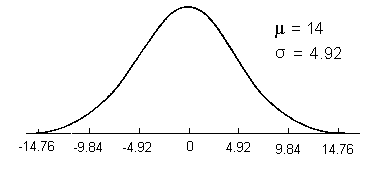
The obtained difference between the means ( = 43.33 - 57.33 = -14.00) is converted to a standard score relative to the theoretical sampling distribution. The resulting value is called a t-score because an estimate of the standard error was used rather than the actual value. The formula used to find t_obs is as follows:

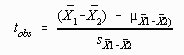
but since = 0.0 under the null hypothesis, the formula may be simplified as follows:

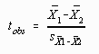
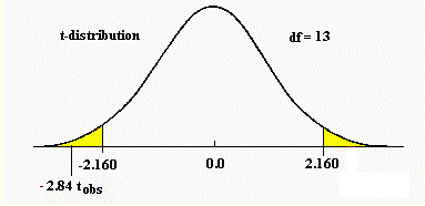
Computing the t_obs using the preceding formula yields 14.00/4.92 = -2.84. The critical value is found in the t tables in Appendix C using N1+N2-2 degrees of freedom. In this case there would be 6 + 9 -2 = 13 degrees of freedom.

The value of for a two-tailed hypothesis test and a =.05 would be ± 2.160. Since the t_obs falls outside the range of the model would be rejected along with the null hypothesis. The alternative hypothesis about the reality of the effect, that females tapped faster than males, would be accepted.

To compute a nested t-test using SPSS, the data for each subject must first be entered with one variable identifying to which group that subject belongs, and a second with the actual score for that subject. In the example data, one variable identifies the gender of the subject and the other identifies the number of finger taps that subject did. The example data file appears as follows:

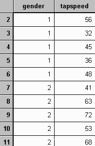
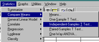
The SPSS package does what I call a nested t-test with the Independent-Samples T Test procedure, which is accessed as follows:

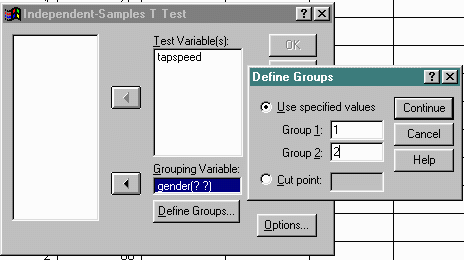
Once selected, the user must describe both the dependent (Test) variable and the independent (Grouping) variable to the procedure. The levels of the grouping variable are further described by clicking on the Define Groups button. Example input to the procedure is presented below:

Clicking on Continue and then OK produces both a table of means

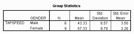
and the results of the nested t-test.

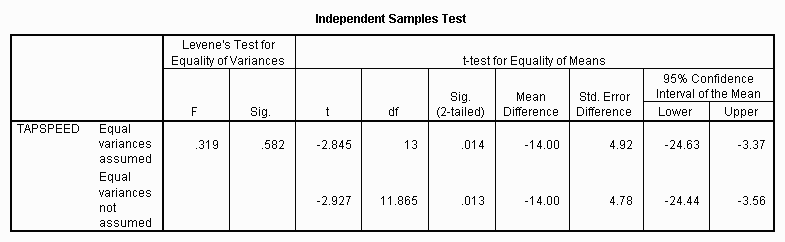
The SPSS output produces more detailed results than those presented earlier in the chapter. The columns titled "Levene's Test for Equality of Variances" presents a test of the assumption that the theoretical variances of the two groups are equal. If this statistic is significant, that is, the value of Sig. is less than .05 (or whatever value for alpha), then some statisticians argue that a different procedure must be used to compute and test for differences between means. The SPSS output gives results of statistical procedures both assuming equal and not equal variances. In the case of the example analysis, the test for equal variances was not significant, indicating that the first t-test would be appropriate.

Note that the procedures described earlier in this chapter produce results within rounding error of those assuming equal variances. When in doubt, the user should probably opt for the more conservative (less likely to find results) t-test not assuming equal variances.

AN EXAMPLE WITHOUT EXPLANATIONS

In an early morning class, one-half the students are given coffee with caffeine and one-half coffee without. The number of times each student yawns during the lecture is recorded with the following results:

Because each student participated in one, and only one, treatment condition, the experiment has subjects nested within treatments.

Step One

Step Two

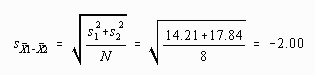
Step Three

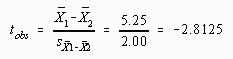
Step Four

Using an a =.01 and a one-tailed t-test, the value of found in the t-tables would be:

= -2.624

Step Five

The null hypothesis is rejected because the value for t_obs is less than the value of . In this case it is possible to say that caffeine had a real effect.

An example of the homework assignment is available.

CONCLUSION

When the experimental design has subjects appearing in one, and only one, of two treatment conditions, a nested t-test is the appropriate analysis. A model of the distribution of differences between sample means under the Null Hypothesis is created and compared with the actual results. If the model is unlikely given the data, the model and the null hypothesis are rejected and the alternative accepted.