Introductory Statistics: Concepts, Models, and Applications
David W. Stockburger
The Pearson Product-Moment Correlation Coefficient (r), or correlation coefficient for short is a measure of the degree of linear relationship between two variables, usually labeled X and Y. While in regression the emphasis is on predicting one variable from the other, in correlation the emphasis is on the degree to which a linear model may describe the relationship between two variables. In regression the interest is directional, one variable is predicted and the other is the predictor; in correlation the interest is non-directional, the relationship is the critical aspect.
The computation of the correlation coefficient is most easily accomplished with the aid of a statistical calculator. The value of r was found on a statistical calculator during the estimation of regression parameters in the last chapter. Although definitional formulas will be given later in this chapter, the reader is encouraged to review the procedure to obtain the correlation coefficient on the calculator at this time.
The correlation coefficient may take on any value between plus and minus one.
![]()
The sign of the correlation coefficient (+ , -) defines the direction of the relationship, either positive or negative. A positive correlation coefficient means that as the value of one variable increases, the value of the other variable increases; as one decreases the other decreases. A negative correlation coefficient indicates that as one variable increases, the other decreases, and vice-versa.
Taking the absolute value of the correlation coefficient measures the strength of the relationship. A correlation coefficient of r=.50 indicates a stronger degree of linear relationship than one of r=.40. Likewise a correlation coefficient of r=-.50 shows a greater degree of relationship than one of r=.40. Thus a correlation coefficient of zero (r=0.0) indicates the absence of a linear relationship and correlation coefficients of r=+1.0 and r=-1.0 indicate a perfect linear relationship.
The correlation coefficient may be understood by various means, each of which will now be examined in turn.
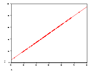
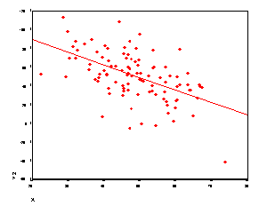
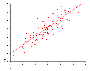
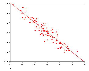
The scatterplots presented below perhaps best illustrate how the correlation coefficient changes as the linear relationship between the two variables is altered. When r=0.0 the points scatter widely about the plot, the majority falling roughly in the shape of a circle. As the linear relationship increases, the circle becomes more and more elliptical in shape until the limiting case is reached (r=1.00 or r=-1.00) and all the points fall on a straight line.
A number of scatterplots and their associated correlation coefficients are presented below in order that the student may better estimate the value of the correlation coefficient based on a scatterplot in the associated computer exercise.
r = 1.00
r = -.54
r = .85
r = -.94
r = .42
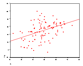
r = -.33
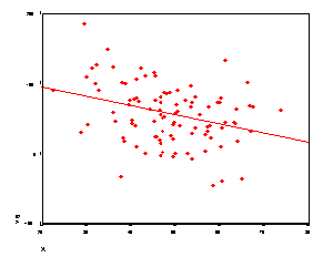
r = .17
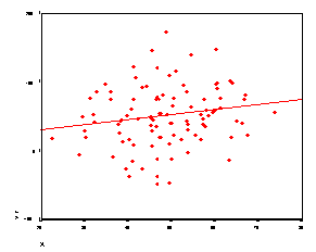
r = .39
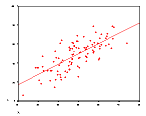
The correlation coefficient is the slope (b) of the regression line when both the X and Y variables have been converted to z-scores. The larger the size of the correlation coefficient, the steeper the slope. This is related to the difference between the intuitive regression line and the actual regression line discussed above.
This interpretation of the correlation coefficient is perhaps best illustrated with an example involving numbers. The raw score values of the X and Y variables are presented in the first two columns of the following table. The second two columns are the X and Y columns transformed using the z-score transformation.
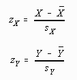
That is, the mean is subtracted from each raw score in the X and Y columns and then the result is divided by the sample standard deviation. The table appears as follows:
|
X |
Y |
zX |
zY |
|
|
12 |
33 |
-1.07 |
-0.61 |
|
|
15 |
31 |
-0.07 |
-1.38 |
|
|
19 |
35 |
-0.20 |
0.15 |
|
|
25 |
37 |
0.55 |
.92 |
|
|
32 |
37 |
1.42 |
.92 |
|
|
20.60 |
34.60 |
0.0 |
0.0 |
|
|
|
8.02 |
2.61 |
1.0 |
1.0 |
There are two points to be made with the above numbers: (1) the correlation coefficient is invariant under a linear transformation of either X and/or Y, and (2) the slope of the regression line when both X and Y have been transformed to z-scores is the correlation coefficient.
Computing the correlation coefficient first with the raw scores X and Y yields r=0.85. Next computing the correlation coefficient with zX and zY yields the same value, r=0.85. Since the z-score transformation is a special case of a linear transformation (X' = a + bX), it may be proven that the correlation coefficient is invariant (doesn't change) under a linear transformation of either X and/or Y. The reader may verify this by computing the correlation coefficient using X and zY or Y and zX. What this means essentially is that changing the scale of either the X or the Y variable will not change the size of the correlation coefficient, as long as the transformation conforms to the requirements of a linear transformation.
The fact that the correlation coefficient is the slope of the regression line when both X and Y have been converted to z-scores can be demonstrated by computing the regression parameters predicting zX from zY or zY from zX. In either case the intercept or additive component of the regression line (a) will be zero or very close, within rounding error. The slope (b) will be the same value as the correlation coefficient, again within rounding error. This relationship may be illustrated as follows:

The squared correlation coefficient (r2) is the proportion of variance in Y that can be accounted for by knowing X. Conversely, it is the proportion of variance in X that can be accounted for by knowing Y.
One of the most important properties of variance is that it may be partitioned into separate additive parts. For example, consider shoe size. The theoretical distribution of shoe size may be presented as follows:
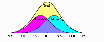
If the scores in this distribution were partitioned into two groups, one for males and one for females, the distributions could be represented as follows:
If one knows the sex of an individual, one knows something about that person's shoe size, because the shoe sizes of males are on the average somewhat larger than females. The variance within each distribution, male and female, is variance that cannot be predicted on the basis of sex, or error variance, because if one knows the sex of an individual, one does not know exactly what that person's shoe size will be.
Rather than having just two levels the X variable will usually have many levels. The preceding argument may be extended to encompass this situation. It can be shown that the total variance is the sum of the variance that can be predicted and the error variance, or variance that cannot be predicted. This relationship is summarized below:

The correlation coefficient squared is equal to the ratio of predicted to total variance:

This formula may be rewritten in terms of the error variance, rather than the predicted variance as follows:
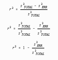
The error variance, s2ERROR, is estimated by the standard error of estimate squared, s2Y.X, discussed in the previous chapter. The total variance (s2TOTAL) is simply the variance of Y, s2Y.The formula now becomes:

Solving for sY.X, and adding a correction factor (N-1)/(N-2), yields the computational formula for the standard error of estimate,

This captures the essential relationship between the correlation coefficient, the variance of Y, and the standard error of estimate. As the standard error of estimate becomes large relative to the total variance, the correlation coefficient becomes smaller. Thus the correlation coefficient is a function of both the standard error of estimate and the total variance of Y. The standard error of estimate is an absolute measure of the amount of error in prediction, while the correlation coefficient squared is a relative measure, relative to the total variance.
The easiest method of computing a correlation coefficient is to use a statistical calculator or computer program. Barring that, the correlation coefficient may be computed using the following formula:

Computation using this formula is demonstrated below on some example data: Computation is rarely done in this manner and is provided as an example of the application of the definitional formula, although this formula provides little insight into the meaning of the correlation coefficient.
|
X |
Y |
zX |
zY |
zXzY |
|
12 |
33 |
-1.07 |
-0.61 |
0.65 |
|
15 |
31 |
-0.07 |
-1.38 |
0.97 |
|
19 |
35 |
-0.20 |
0.15 |
-0.03 |
|
25 |
37 |
0.55 |
.92 |
0.51 |
|
32 |
37 |
1.42 |
.92 |
1.31 |
|
SUM = |
3.40 |

A convenient way of summarizing a large number of correlation coefficients is to put them in in a single table, called a correlation matrix. A Correlation Matix is a table of all possible correlation coefficients between a set of variables. For example, suppose a questionnaire of the following form (Reed, 1983) produced a data matrix as follows.
AGE - What is your age? _____
KNOW - Number of correct answers out of 10 possible to a Geology quiz which consisted of correctly locating 10 states on a state map of the United States.
VISIT - How many states have you visited? _____
COMAIR - Have you ever flown on a commercial airliner? _____
SEX - 1 = Male, 2 = Female
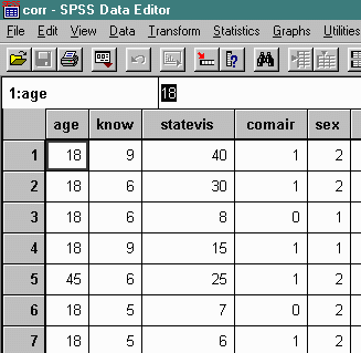
Since there are five questions on the example questionnaire there are 5 * 5 = 25 different possible correlation coefficients to be computed. Each computed correlation is then placed in a table with variables as both rows and columns at the intersection of the row and column variable names. For example, one could calculate the correlation between AGE and KNOWLEDGE, AGE and STATEVIS, AGE and COMAIR, AGE and SEX, KNOWLEDGE and STATEVIS, etc., and place then in a table of the following form.
One would not need to calculate all possible correlation coefficients, however, because the correlation of any variable with itself is necessarily 1.00. Thus the diagonals of the matrix need not be computed. In addition, the correlation coefficient is non-directional. That is, it doesn't make any difference whether the correlation is computed between AGE and KNOWLEDGE with AGE as X and KNOWLEDGE as Y or KNOWLDEGE as X and AGE as Y. For this reason the correlation matrix is symmetrical around the diagonal. In the example case then, rather than 25 correlation coefficients to compute, only 10 need be found, 25 (total) - 5 (diagonals) - 10 (redundant because of symmetry) = 10 (different unique correlation coefficients).
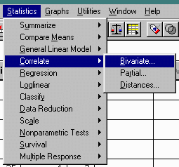
To calculate a correlation matrix using SPSS select CORRELATIONS and BIVARIATE as follows:
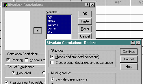
Select the variables that are to be included in the correlation matrix as follows. In this case all variables will be included, and optional means and standard deviations will be output.
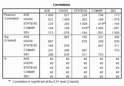
The results of the preceding are as follows:
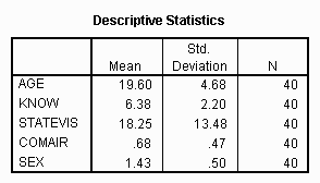
Interpretation of the data analysis might proceed as follows. The table of means and standard deviations indicates that the average Psychology 121 student who filled out this questionnaire was about 19 years old, could identify slightly more than six states out of ten, and had visited a little over 18 of the 50 states. The majority (67%) have flown on a commercial airplane and there were fewer females (43%) than males.
The analysis of the correlation matrix indicates that few of the observed relationships were very strong. The strongest relationship was between the number of states visited and whether or not the student had flown on a commercial airplane (r=.42) which indicates that if a student had flown he/she was more likely to have visited more states. This is because of the positive sign on the correlation coefficient and the coding of the commercial airplane question (0=NO, 1=YES). The positive correlation means that as X increases, so does Y: thus, students who responded that they had flown on a commercial airplane visited more states on the average than those who hadn't.
Age was positively correlated with number of states visited (r=.22) and flying on a commercial airplane (r=.19) with older students more likely both to have visited more states and flown, although the relationship was not very strong. The greater the number of states visited, the more states the student was likely to correctly identify on the map, although again relationship was weak (r=.28). Note that one of the students who said he had visited 48 of the 50 states could identify only 5 of 10 on the map.
Finally, sex of the participant was slightly correlated with both age, (r=.17) indicating that females were slightly older than males, and number of states visited (r=-.16), indicating that females visited fewer states than males These conclusions are possible because of the sign of the correlation coefficient and the way the sex variable was coded: 1=male 2=female. When the correlation with sex is positive, females will have more of whatever is being measured on Y. The opposite is the case when the correlation is negative.
Correct interpretation of a correlation coefficient requires the assumption that both variables, X and Y, meet the interval property requirements of their respective measurement systems. Calculators and computers will produce a correlation coefficient regardless of whether or not the numbers are "meaningful" in a measurement sense.
As discussed in the chapter on Measurement, the interval property is rarely, if ever, fully satisfied in real applications. There is some difference of opinion among statisticians about when it is appropriate to assume the interval property is met. My personal opinion is that as long as a larger number means that the object has more of something or another, then application of the correlation coefficient is useful, although the potentially greater deviations from the interval property must be interpreted with greater caution. When the data is clearly nominal categorical with more than two levels (1=Protestant, 2=Catholic, 3=Jewish, 4=Other), application of the correlation coefficient is clearly inappropriate.
An exception to the preceding rule occurs when the nominal categorical scale is dichotomous, or has two levels (1=Male, 2=Female). Correlation coefficients computed with data of this type on either the X and/or Y variable may be safely interpreted because the interval property is assumed to be met for these variables. Correlation coefficients computed using data of this type are sometimes given special, different names, but since they seem to add little to the understanding of the meaning of the correlation coefficient, they will not be presented.
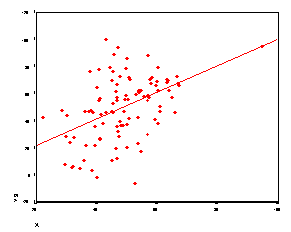
An outlier is a score that falls outside the range of the rest of the scores on the scatterplot. For example, if age is a variable and the sample is a statistics class, an outlier would be a retired individual. Depending upon where the outlier falls, the correlation coefficient may be increased or decreased.
An outlier which falls near where the regression line would normally fall would necessarily increase the size of the correlation coefficient, as seen below.
r = .457
An outlier that falls some distance away from the original regression line would decrease the size of the correlation coefficient, as seen below:
r = .336
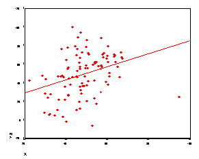
The effect of the outliers on the above examples is somewhat muted because the sample size is fairly large (N=100). The smaller the sample size, the greater the effect of the outlier. At some point the outlier will have little or no effect on the size of the correlation coefficient.
When a researcher encounters an outlier, a decision must be made whether to include it in the data set. It may be that the respondent was deliberately malingering, giving wrong answers, or simply did not understand the question on the questionnaire. On the other hand, it may be that the outlier is real and simply different. The decision whether to include or not include an outlier remains with the researcher; he or she must justify deleting any data to the reader of a technical report, however. It is suggested that the correlation coefficient be computed and reported both with and without the outlier if there is any doubt about whether or not it is real data. In any case, the best way of spotting an outlier is by drawing the scatterplot.
No discussion of correlation would be complete without a discussion of causation. It is possible for two variables to be related (correlated), but not have one variable cause another.
For example, suppose there exists a high correlation between the number of popsicles sold and the number of drowning deaths. Does that mean that one should not eat popsicles before one swims? Not necessarily. Both of the above variable are related to a common variable, the heat of the day. The hotter the temperature, the more popsicles sold and also the more people swimming, thus the more drowning deaths. This is an example of correlation without causation.
Much of the early evidence that cigarette smoking causes cancer was correlational. It may be that people who smoke are more nervous and nervous people are more susceptible to cancer. It may also be that smoking does indeed cause cancer. The cigarette companies made the former argument, while some doctors made the latter. In this case I believe the relationship is causal and therefore do not smoke.
Sociologists are very much concerned with the question of correlation and causation because much of their data is correlational. Sociologists have developed a branch of correlational analysis, called path analysis, precisely to determine causation from correlations (Blalock, 1971). Before a correlation may imply causation, certain requirements must be met. These requirements include: (1) the causal variable must temporally precede the variable it causes, and (2) certain relationships between the causal variable and other variables must be met.
If a high correlation was found between the age of the teacher and the students' grades, it does not necessarily mean that older teachers are more experienced, teach better, and give higher grades. Neither does it necessarily imply that older teachers are soft touches, don't care, and give higher grades. Some other explanation might also explain the results. The correlation means that older teachers give higher grades; younger teachers give lower grades. It does not explain why it is the case.
A simple correlation may be interpreted in a number of different ways: as a measure of linear relationship, as the slope of the regression line of z-scores, and as the correlation coefficient squared as the proportion of variance accounted for by knowing one of the variables. All the above interpretations are correct and in a certain sense mean the same thing.
A number of qualities which might effect the size of the correlation coefficient were identified. They included missing parts of the distribution, outliers, and common variables. Finally, the relationship between correlation and causation was discussed.