A linear transformation is a transformation of the form X' = a + bX. If a measurement system approximated an interval scale before the linear transformation, it will approximate it to the same degree after the linear transformation. Other properties of the distribution are similarly unaffected. For example, if a distribution was positively skewed before the transformation, it will be positively skewed after.

The symbols in the transformation equation, X'_i = a + bX_i, have the following meaning. The raw score is denoted by X_i, the score after the transformation is denoted by X'_i, read X prime or X transformed. The "b" is the multiplicative component of the linear transformation, sometimes called the slope, and the "a" is the additive component, sometimes referred to as the intercept. The "a" and "b" of the transformation are set to real values to specify a transformation.

The transformation is performed by first multiplying every score value by the multiplicative component "b" and then adding the additive component "a" to it. For example, the following set of data is linearly transformed with the transformation X'_i = 20 + 3*X_i, where a = 20 and b = 3.

Linear Transformation - a=20, b=3

The score value of 12, for example, is transformed first by multiplication by 3 to get 36 and then this product is added to 20 to get the result of 56.

The effect of the linear transformation on the mean and standard deviation of the scores is of considerable interest. For that reason, both, the additive and multiplicative components, of the transformation will be examined separately for their relative effects.

THE ADDITIVE COMPONENT

If the multiplicative component is set equal to one, the linear transformation becomes X' = a + X, so that the effect of the additive component may be examined. With this transformation, a constant is added to every score. An example additive transformation is shown below:

Linear Transformation - a=20, b=1

The transformed mean, , is equal to the original mean, , plus the transformation constant, in this case a=20. The standard deviation does not change. It is as if the distribution was lifted up and placed back down to the right or left, depending upon whether the additive component was positive or negative. The effect of the additive component is graphically presented below.

THE MULTIPLICATIVE COMPONENT

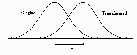
The effect of the multiplicative component "b" may be examined separately if the additive component is set equal to zero. The transformation equation becomes X' = bX, which is the type of transformation done when the scale is changed, for example from feet to inches. In that case, the value of b would be equal to 12 because there are 12 inches to the foot. Similarly, transformations to and from the metric system, i.e. pounds to kilograms, and back again are multiplicative transformations.

An example multiplicative transformation is presented below, where b=3:

Linear Transformation - a=0, b=3

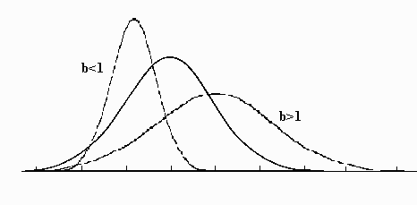
Note that both the mean and the standard deviation of the transformed scores are three times their original value, which is precisely the amount of the multiplicative component. The multiplicative component, then, effects both the mean and standard deviation by its size, as illustrated below:

LINEAR TRANSFORMATIONS - EFFECT ON MEAN AND STANDARD DEVIATION

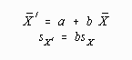
Putting the separate effects of the additive and multiplicative components together in a linear transformation, it would be expected that the standard deviation would be effected only by the multiplicative component and the mean by both. The following two equations express the relationships:

For example, in the original distribution and the linear transformation of X' = 20 + 3*X, the transformed mean and standard deviation would be expected to be:

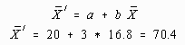
If the transformation is done and the new mean and standard deviation computed, this is exactly what is found, within rounding error.

Linear Transformation - a=20, b=3

The question students most often ask at this point is where do the values of "a" and "b" come from. "Are you just making them up as you go along?" is the most common question. That is exactly what has been done up to this point in time. Now the procedure for finding a and b such that the new mean and standard deviation will be a given value will be presented.

LINEAR TRANSFORMATIONS - FINDING a AND b GIVEN AND s_X'

Suppose that the original scores were raw scores from an intelligence test. Historically, IQ's or intelligence test scores have a mean of 100 and a standard deviation of either 15 or 16, depending upon the test selected. In order to convert the raw scores to IQ scores on an IQ scale, a linear transformation is performed such that the transformed mean and standard deviation are 100 and 16, respectively. The problem is summarized in the following table:

Linear Transformation - a=?, b=?

This problem may be solved by first recalling how the mean and standard deviation are effected by the linear transformation:

In these two equations are two unknowns, a and b. Because these equations are independent, they may be solved for a and b in the following manner. First, solving for b by dividing both sides of the equation by s_X produces:

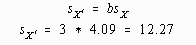
Thus the value of "b" is found by dividing the new or transformed standard deviation by the original standard deviation.

After finding the value of b, the value of a may be found in the following manner:

In this case the product of the value of b times the original mean is subtracted from the new or transformed mean.

These two equations can be summarized as follows:

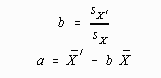
Application of these equations to the original problem where = 100 and s_X' = 16 produces the following results:

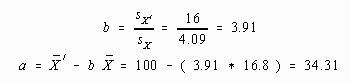
Plugging these values into the original problem produces the desired results, within rounding error.

Linear Transformation - a=34.31, b=3.91

The transformed scores are now on an IQ scale. Before they may be considered as IQ's, however, the test must be validated as an IQ test. If the original test had little or nothing to do with intelligence, then the IQ's which result from a linear transformation such as the one above would be meaningless.

Using the above procedure, a given distribution with a given mean and standard deviation may be transformed into another distribution with any given mean and standard deviation. In order to turn this flexibility into some kind of order, some kind of standard scale has to be selected. The IQ scale is one such standard, but its use is pretty well limited to intelligence tests. Another standard is the T-distribution, where scores are transformed into a scale with a mean of 50 and a standard deviation of 10. This transformation has the advantage of always being positive and between the values of 1 and 100. Another transformation is a stanine transformation where scores are transformed to a distribution with a mean of 5 and a standard deviation of 2. In this transformation the decimals are dropped, so a score of an integer value between 1 and 9 is produced. The Army used this transformation because the results could fit on a single column on a computer card.

STANDARD SCORES OR Z-SCORES

Another possible transformation is so important and widely used that it deserves an entire section to itself. It is the standard score or z-score transformation. The standard score transformation is a linear transformation such that the transformed mean and standard deviation are 0 and 1 respectively. The selection of these values was somewhat arbitrary, but not without some reason.

Transformation to z-scores could be accomplished using the procedure described in the earlier section to convert any distribution to a distribution with a given mean and standard deviation, in this case 0 and 1. This is demonstrated below with the example data.

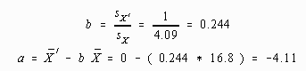
Linear Transformation - a=-4.11, b=0.244

Note that the transformed mean and standard deviation are within rounding error of the desired figures.

Using a little algebra, the computational formulas to convert raw scores to z-scores may be simplified. When converting to standard scores (=0 and s_X'=1.0), the value of a can be found by the following:

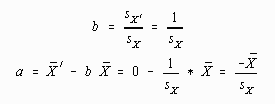
The value for b can then be found by substituting these values into the linear transformation equation:

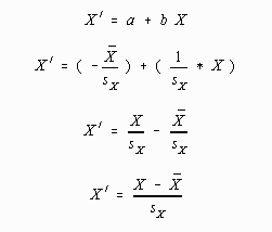
The last result is a computationally simpler version of the standard score transformation. All this algebra was done to demonstrate that the standard score or z-score transformation was indeed a type of linear transformation. If a student is unable to follow the mathematics underlying the algebraic transformation, he or she will just have to "Believe!" In any case, the formula for converting to z-scores is:

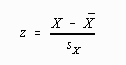
(Note that the "z" has replaced the "X'")

Application of this computational formula to the example data yields:

Z-score Transformation

Note that the two procedures produce almost identical results, except that the computational formula is slightly more accurate. Because of the increased accuracy and ease of computation, it is the method of choice in this case.

FINDING LINEAR TRANSFORMATIONS USING SPSS

All of the transformations described in this chapter could be done using the COMPUTE command on SPSS. The following presents a series of COMPUTE commands pasted into a SYNTAX file using SPSS to perform all the transformations previously described in this chapter.

COMPUTE AddTrans = 20 + x .
COMPUTE MulTrans = 3 * x .
COMPUTE LinTrans = 20 + ( 3 * x ) .
COMPUTE IQTrans = 34.31 + ( 3.91 * x ) .
COMPUTE Z1Trans = -4.11 + ( 0.244 * x ) .
COMPUTE Z2Trans = ( x - 16.8 ) / 4.09 .
COMPUTE Perrank = CDFNORM(Z2Trans) .
EXECUTE .

The variables that resulted were printed using the CASE SUMMARIES command.

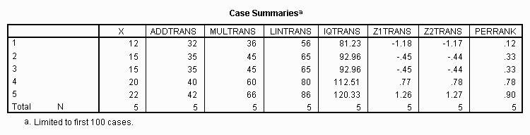
The means and standard deviations of this file were found using the DESCRIPTIVES command.

CONCLUSION AND SUMMARY

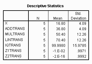
Transformations are performed to interpret and compare raw scores. Of the two types of transformations described in this text, percentile ranks are preferred to interpret scores to the lay public, because they are more easily understood. Because of the unfortunate property of destroying the interval property of the scale, the statistician uses percentile rank transformations with reluctance. Linear transformations are preferred because the interval property of the measurement system is not disturbed.

Using a linear transformation, a distribution with a given mean and standard deviation may be transformed into another distribution with a different mean and standard deviation. Several standards for the mean and standard deviation were discussed, but standard scores or z-scores are generally the preferred transformation. The z-score transformation is a linear transformation with a transformed mean of 0 and standard deviation of 1.0. Computational procedures were provided for this transformation.

Standard scores could be converted to percentile ranks by use of the standard normal curve tables. Computation of percentile ranks using this method required additional assumptions about the nature of the world and had the same unfortunate property as percentile ranks based on the sample.