Introductory Statistics: Concepts, Models, and Applications
David W. Stockburger
As discussed in the previous chapter, the normal curve is one of a number of possible models of probability distributions. Because it is widely used and an important theoretical tool, it is given special status as a separate chapter.
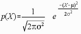
The normal curve is not a single curve, rather it is an infinite number of possible curves, all described by the same algebraic expression:

Upon viewing this expression for the first time the initial reaction of the student is usually to panic. Don't. In general it is not necessary to "know" this formula to appreciate and use the normal curve. It is, however, useful to examine this expression for an understanding of how the normal curve operates.
First, some symbols in the expression are simply numbers. These symbols include "2", "P ", and "e". The latter two are rational numbers that are very long, P equaling 3.1416... and e equaling 2.81.... As discussed in the chapter on the review of algebra, it is possible to raise a "funny number", in this case "e", to a "funny power".
The second set of symbols which are of some interest includes the symbol "X", which is a variable corresponding to the score value. The height of the curve at any point is a function of X.
Thirdly, the final two symbols in the equation, "m " and "d " are called PARAMETERS, or values which, when set to particular numbers, define which of the infinite number of possible normal curves with which one is dealing. The concept of parameters is very important and considerable attention will be given them in the rest of this chapter.
The normal curve is called a family of distributions. Each member of the family is determined by setting the parameters (m and d ) of the model to a particular value (number). Because the m parameter can take on any value, positive or negative, and the s parameter can take on any positive value, the family of normal curves is quite large, consisting of an infinite number of members. This makes the normal curve a general-purpose model, able to describe a large number of naturally occurring phenomena, from test scores to the size of the stars.
All the members of the family of normal curves, although different, have a number of properties in common. These properties include: shape, symmetry, tails approaching but never touching the X-axis, and area under the curve.
All members of the family of normal curves share the same bell shape, given the X-axis is scaled properly. Most of the area under the curve falls in the middle. The tails of the distribution (ends) approach the X-axis but never touch, with very little of the area under them.
All members of the family of normal curves are bilaterally symmetrical. That is, if any normal curve was drawn on a two-dimensional surface (a piece of paper), cut out, and folded through the third dimension, the two sides would be exactly alike. Human beings are approximately bilaterally symmetrical, with a right and left side.
All members of the family of normal curves have tails that approach, but never touch, the X-axis. The implication of this property is that no matter how far one travels along the number line, in either the positive or negative direction, there will still be some area under any normal curve. Thus, in order to draw the entire normal curve one must have an infinitely long line. Because most of the area under any normal curve falls within a limited range of the number line, only that part of the line segment is drawn for a particular normal curve.
All members of the family of normal curves have a total area of one (1.00) under the curve, as do all probability models or models of frequency distributions. This property, in addition to the property of symmetry, implies that the area in each half of the distribution is .50 or one half.
Because area under a curve may seem like a strange concept to many introductory statistics students, a short intermission is proposed at this point to introduce the concept.
Area is a familiar concept. For example, the area of a square is s2, or side squared; the area of a rectangle is length times height; the area of a right triangle is one-half base times height; and the area of a circle is P * r2. It is valuable to know these formulas if one is purchasing such things as carpeting, shingles, etc.
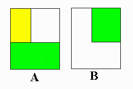
Areas may be added or subtracted from one another to find some resultant area. For example, suppose one had an L-shaped room and wished to purchase new carpet. One could find the area by taking the total area of the larger rectangle and subtracting the area of the rectangle that was not needed, or one could divide the area into two rectangles, find the area of each, and add the areas together. Both procedures are illustrated below:
Finding the area under a curve poses a slightly different problem. In some cases there are formulas which directly give the area between any two points; finding these formulas are what integral calculus is all about. In other cases the areas must be approximated. All of the above procedures share a common theoretical underpinning, however.
Suppose a curve was divided into equally spaced intervals on the X-axis and a rectangle drawn corresponding to the height of the curve at any of the intervals. The rectangles may be drawn either smaller that the curve, or larger, as in the two illustrations below:


In either case, if the areas of all the rectangles under the curve were added together, the sum of the areas would be an approximation of the total area under the curve. In the case of the smaller rectangles, the area would be too small; in the case of the latter, they would be too big. Taking the average would give a better approximation, but mathematical methods provide a better way.
A better approximation may be achieved by making the intervals on the X-axis smaller. Such an approximations is illustrated below, more closely approximating the actual area under the curve.

The actual area of the curve may be calculated by making the intervals infinitely small (no distance between the intervals) and then computing the area. If this last statement seems a bit bewildering, you share the bewilderment with millions of introductory calculus students. At this point the introductory statistics student must say "I believe" and trust the mathematician or enroll in an introductory calculus course.
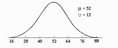
The standard procedure for drawing a normal curve is to draw a bell-shaped curve and an X-axis. A tick is placed on the X-axis in corresponding to the highest point (middle) of the curve. Three ticks are then placed to both the right and left of the middle point. These ticks are equally spaced and include all but a very small portion under the curve. The middle tick is labeled with the value of m ; sequential ticks to the right are labeled by adding the value of d . Ticks to the left are labeled by subtracting the value of d from m for the three values. For example, if m =52 and d =12, then the middle value would be labeled with 52, points to the right would have the values of 64 (52 + 12), 76, and 88, and points to the left would have the values 40, 28, and 16. An example is presented below:
Differences in members of the family of normal curves are a direct result of differences in values for parameters. The two parameters, m and d , each change the shape of the distribution in a different manner.
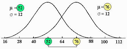
The first, m , determines where the midpoint of the distribution falls. Changes in m , without changes in d , result in moving the distribution to the right or left, depending upon whether the new value of m was larger or smaller than the previous value, but does not change the shape of the distribution. An example of how changes in m affect the normal curve are presented below:
Changes in the value of d , on the other hand, change the shape of the distribution without affecting the midpoint, because d affects the spread or the dispersion of scores. The larger the value of d , the more dispersed the scores; the smaller the value, the less dispersed. Perhaps the easiest way to understand how d affects the distribution is graphically. The distribution below demonstrates the effect of increasing the value of d :
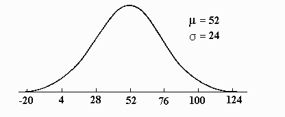
Since this distribution was drawn according to the procedure described earlier, it appears similar to the previous normal curve, except for the values on the X-axis. This procedure effectively changes the scale and hides the real effect of changes in d . Suppose the second distribution was drawn on a rubber sheet instead of a sheet of paper and stretched to twice its original length in order to make the two scales similar. Drawing the two distributions on the same scale results in the following graphic:
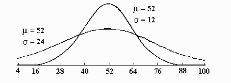
Note that the shape of the second distribution has changed dramatically, being much flatter than the original distribution. It must not be as high as the original distribution because the total area under the curve must be constant, that is, 1.00. The second curve is still a normal curve; it is simply drawn on a different scale on the X-axis.
A different effect on the distribution may be observed if the size of d is decreased. Below the new distribution is drawn according to the standard procedure for drawing normal curves:
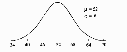
Now both distributions are drawn on the same scale, as outlined immediately above, except in this case the sheet is stretched before the distribution is drawn and then released in order that the two distributions are drawn on similar scales:
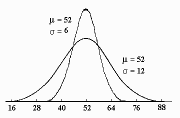
Note that the distribution is much higher in order to maintain the constant area of 1.00, and the scores are much more closely clustered around the value of m , or the midpoint, than before.
An interactive exercise is provided to demonstrate how the normal curve changes as a function of changes in m and d . The exercise starts by presenting a curve with m = 70 and d = 10. The student may change the value of m from 50 to 90 by moving the scroll bar on the bottom of the graph. In a similar manner, the value of d can be adjusted from 5 to 15 by changing the scroll bar on the right side of the graph.
Suppose that when ordering shoes to restock the shelves in the store one knew that female shoe sizes were normally distributed with m = 7.0 and d = 1.1. Don't worry about where these values came from at this point, there will be plenty about that later. If the area under this distribution between 7.75 and 8.25 could be found, then one would know the proportion of size eight shoes to order. The values of 7.75 and 8.25 are the real limits of the interval of size eight shoes.
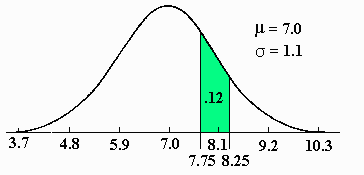
Finding the areas on the curve above is easy; simply enter the value of mu, sigma, and the score or scores into the correct boxes and click on a button on the display and the area appears. The following is an example of the use of the Normal Curve Area program and the reader should verify how the program works by entering the values in a separate screen.
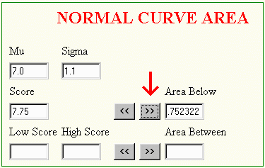
To find the area below 7.75 on a normal curve with mu =7.0 and sigma=1.1 enter the following information and click on the button pointed to with the red arrow.
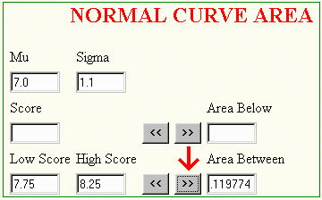
To find the area between scores, enter the low and high scores in the lower boxes and click on the box pointing to the "Area Between."
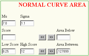
The area above a given score could be found on the above program by subtracting the area below the score from 1.00, the total area under the curve, or by entering the value as a "Low Score" on the bottom boxes and a corresponding very large value for a "High Score." The following illustrates the latter method. The value of "12" is more than three sigma units from the mu of 7.0, so the area will include all but the smallest fraction of the desired area.
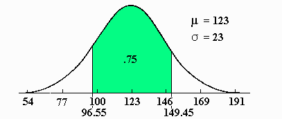
In some applications of the normal curve, it will be necessary to find the scores that cut off some proportion or percentage of area of the normal distribution. For example, suppose one wished to know what two scores cut off the middle 75% of a normal distribution with m = 123 and d = 23. In order to answer questions of this nature, the Normal Curve Area program can be used as follows:
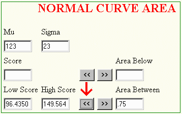
The results can be visualized as follows:
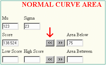
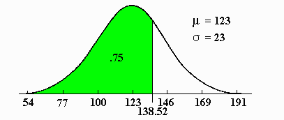
In a similar manner, the score value which cuts of the bottom proportion of a given normal curve can be found using the program. For example a score of 138.52 cuts off .75 of a normal curve with mu=123 and sigma=23. This area was found using Normal Curve Area program in the following manner.
The results can be visualized as follows:
The standard normal curve is a member of the family of normal curves with m = 0.0 and d = 1.0. The value of 0.0 was selected because the normal curve is symmetrical around m and the number system is symmetrical around 0.0. The value of 1.0 for d is simply a unit value. The X-axis on a standard normal curve is often relabeled and called Z scores.
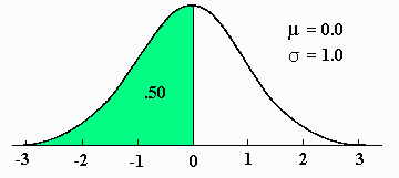
There are three areas on a standard normal curve that all introductory statistics students should know. The first is that the total area below 0.0 is .50, as the standard normal curve is symmetrical like all normal curves. This result generalizes to all normal curves in that the total area below the value of mu is .50 on any member of the family of normal curves.
The second area that should be memorized is between Z-scores of -1.00 and +1.00. It is .68 or 68%.
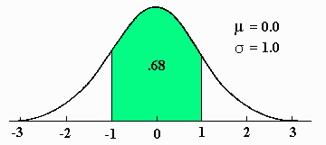
The total area between plus and minus one sigma unit on any member of the family of normal curves is also .68.
The third area is between Z-scores of -2.00 and +2.00 and is .95 or 95%.
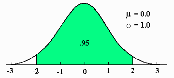
This area (.95) also generalizes to plus and minus two sigma units on any normal curve.
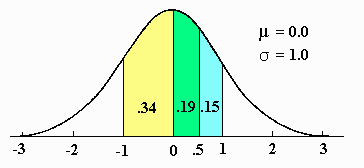
Knowing these areas allow computation of additional areas. For example, the area between a Z-score of 0.0 and 1.0 may be found by taking 1/2 the area between Z-scores of -1.0 and 1.0, because the distribution is symmetrical between those two points. The answer in this case is .34 or 34%. A similar logic and answer is found for the area between 0.0 and -1.0 because the standard normal distribution is symmetrical around the value of 0.0.
The area below a Z-score of 1.0 may be computed by adding .34 and .50 to get .84. The area above a Z-score of 1.0 may now be computed by subtracting the area just obtained from the total area under the distribution (1.00), giving a result of 1.00 - .84 or .16 or 16%.
The area between -2.0 and -1.0 requires additional computation. First, the area between 0.0 and -2.0 is 1/2 of .95 or .475. Because the .475 includes too much area, the area between 0.0 and -1.0 (.34) must be subtracted in order to obtain the desired result. The correct answer is .475 - .34 or .135.
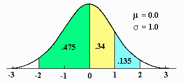
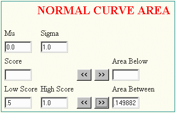
Using a similar kind of logic to find the area between Z-scores of .5 and 1.0 will result in an incorrect answer because the curve is not symmetrical around .5. The correct answer must be something less than .17, because the desired area is on the smaller side of the total divided area. Because of this difficulty, the areas can be found using the program included in this text. Entering the following information will produce the correct answer
The result can be seen graphically in the following:
The following formula is used to transform a given normal distribution into the standard normal distribution. It was much more useful when area between and below a score was only contained in tables of the standard normal distribution. It is included here for both historical reasons and because it will appear in a different form later in this text.

The normal curve is an infinite number of possible probability models called a family of distributions. Each member of the family is described by setting the parameters (m and d ) of the distribution to particular values. The members of the family are similar in that they share the same shape, are symmetrical, and have a total area underneath of 1.00. They differ in where the midpoint of the distribution falls, determined by m , and in the variability of scores around the midpoint, determined by d . The area between any two scores and the scores which cut off a given area on any given normal distribution can be easily found using the program provided with this text